L01 · Intro
L01 · Intro
Topic: intro · 28 pages
EECS 4340 — Computer Hardware Design
Course Staff Introductions
Show slide text
Course Staff Introductions
Instructor: Tanvir Ahmed Khan, tk3070@columbia.edu
Research interests:
- Efficient and reliable data center processing
- Computer architecture, compilers, and operating systems
Class info:
Logistical slide introducing the instructor (Prof. Tanvir Ahmed Khan) and the EECS 4340 Courseworks site. The research interests — datacenter efficiency and the boundary between architecture, compilers, and OS — frame why later lectures emphasize branch prediction, caches, and out-of-order execution from a modern, server-class workload perspective.
Student Introductions
Show slide text
Student Introductions
Introduce yourself: name, level of study (e.g., 1st year CE MS, CS Senior), anything you want to share
Enrollment status:
- Definitely take it
- Unsure if I want to continue
- Waitlisted
Goals from this course:
- What attracted you to computer hardware design?
- Do you have any experience relevant to computer hardware design?
- What do you expect from this course?
- Build background for an industry job
- Complete course requirements
An ice-breaker prompting students to declare enrollment intent (definitely taking, unsure, or waitlisted) and personal goals. The goal-setting questions matter for course pacing because Prof. Khan calibrates project depth against how many students plan to use the material industrially versus as a requirement check-off.
Architecture, Organization, Implementation
Show slide text
Architecture, Organization, Implementation
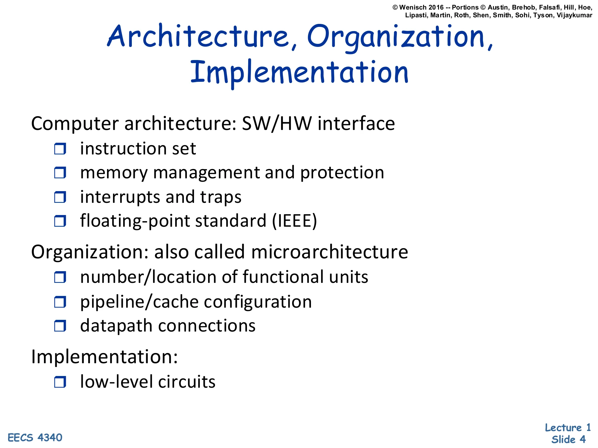
Computer architecture: SW/HW interface
- instruction set
- memory management and protection
- interrupts and traps
- floating-point standard (IEEE)
Organization: also called microarchitecture
- number/location of functional units
- pipeline/cache configuration
- datapath connections
Implementation:
- low-level circuits
This slide draws the textbook three-level distinction that frames the rest of EECS 4340. Architecture is the contract between software and hardware: the ISA, memory model, exception/trap behavior, and standards like precise interrupts or IEEE-754 floating point. Two CPUs implementing the same architecture run the same binary. Organization (a.k.a. microarchitecture) is how a particular CPU realizes that contract — how many ALUs and load/store units it has, how its caches are sized and laid out, whether it pipelines or executes out of order, and how the TLB connects to the L1. Two CPUs sharing an ISA can differ wildly here (e.g., an Apple M-series core vs. an Intel E-core both run x86_64 binaries via different organizations — well, x86 on M is via translation, but the point about Intel P vs. E cores is direct). Implementation is the physical realization: transistor sizing, clock distribution, voltage domains, layout. The three layers separate concerns so a single ISA can survive decades of organization and implementation changes.
What Is EECS 4340 All About?
Show slide text
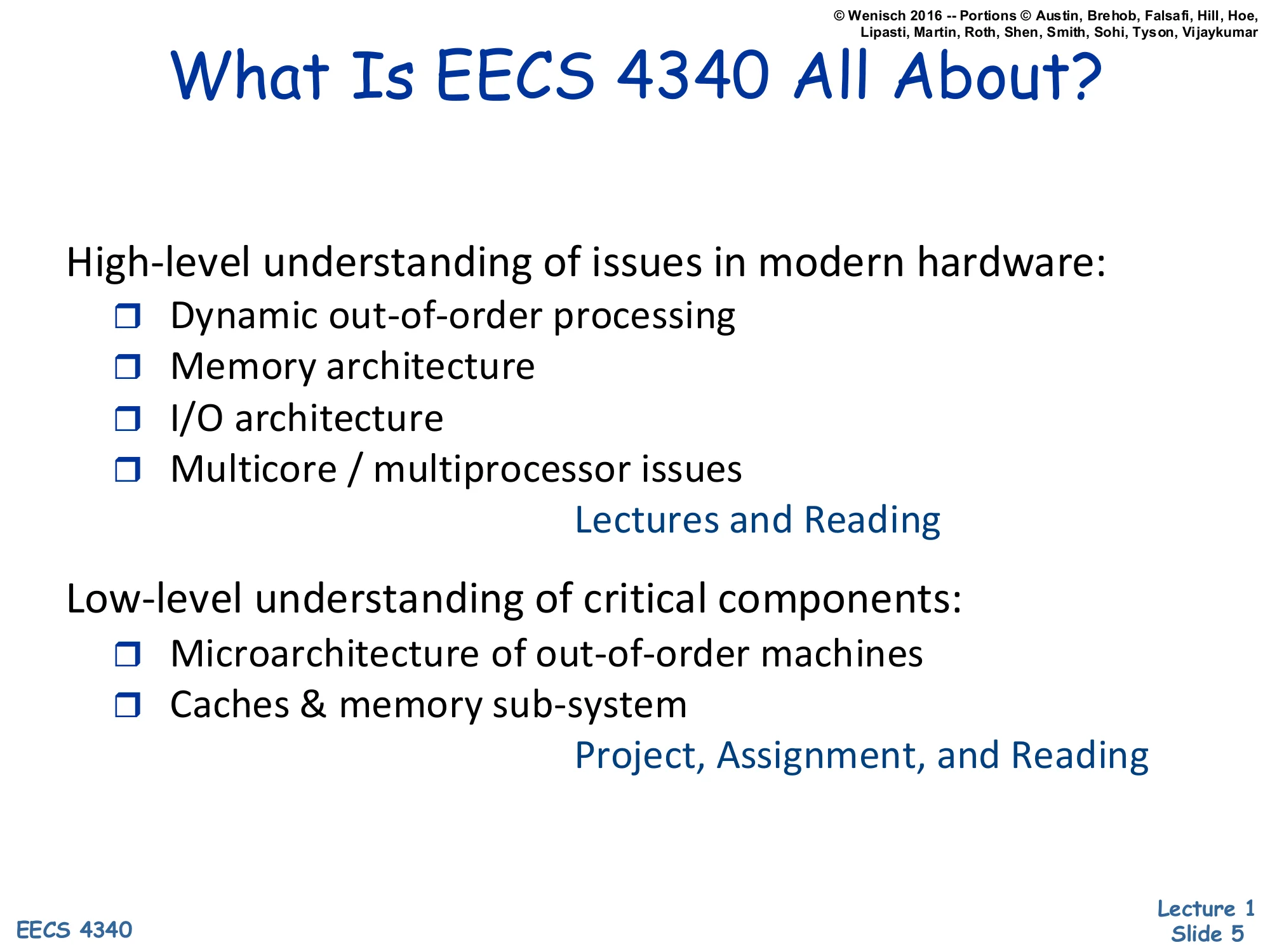
What Is EECS 4340 All About?
High-level understanding of issues in modern hardware:
- Dynamic out-of-order processing
- Memory architecture
- I/O architecture
- Multicore / multiprocessor issues
Lectures and Reading
Low-level understanding of critical components:
- Microarchitecture of out-of-order machines
- Caches & memory sub-system
Project, Assignment, and Reading
Roadmap of the course split into two depths. The high-level half is delivered through lectures and reading and surveys dynamic out-of-order processing, memory architecture, I/O, and multicore/multiprocessor issues — essentially the four chapters of a modern Hennessy & Patterson. The low-level half is hands-on: projects, lab assignments, and reading drill into the actual microarchitecture of ROB-based out-of-order machines and the cache hierarchy. The slide also signals course balance: lectures focus on breadth, but the project (35% of the grade) is where depth is graded.
Meeting Times
Show slide text
Meeting Times
Lecture and Lab
- Monday and Wednesday from 8:40 AM to 9:55 AM
Office Hours
- See the time and location on the course website, it may change
Logistics: lecture and lab are both scheduled Monday/Wednesday 8:40–9:55 AM, and office hours are pinned to the course website because they may shift mid-semester.
Who Should Take EECS 4340?
Show slide text
Who Should Take EECS 4340?
Seniors (ambitious Juniors) & Graduate Students
- Computer architects to be
- Computer hardware designers
- Computer system designers
- Those interested in computer systems
Required Background
- Basic digital logic and computer organization (EECS 3827)
- Verilog/VHDL experience helpful (covered in labs)
Audience and prerequisites. The intended student is a senior or graduate student aiming at architecture, hardware, or systems work. Prerequisite is EECS 3827 (basic digital logic and computer organization) — that course is where students learn registers, FSMs, single-cycle datapaths, and basic memory hierarchy, all of which EECS 4340 builds on. Verilog/VHDL is preferred but not strictly required because the labs walk through it; this matters for the open-ended Verilog project that dominates the grade.
Grading
Show slide text
Grading
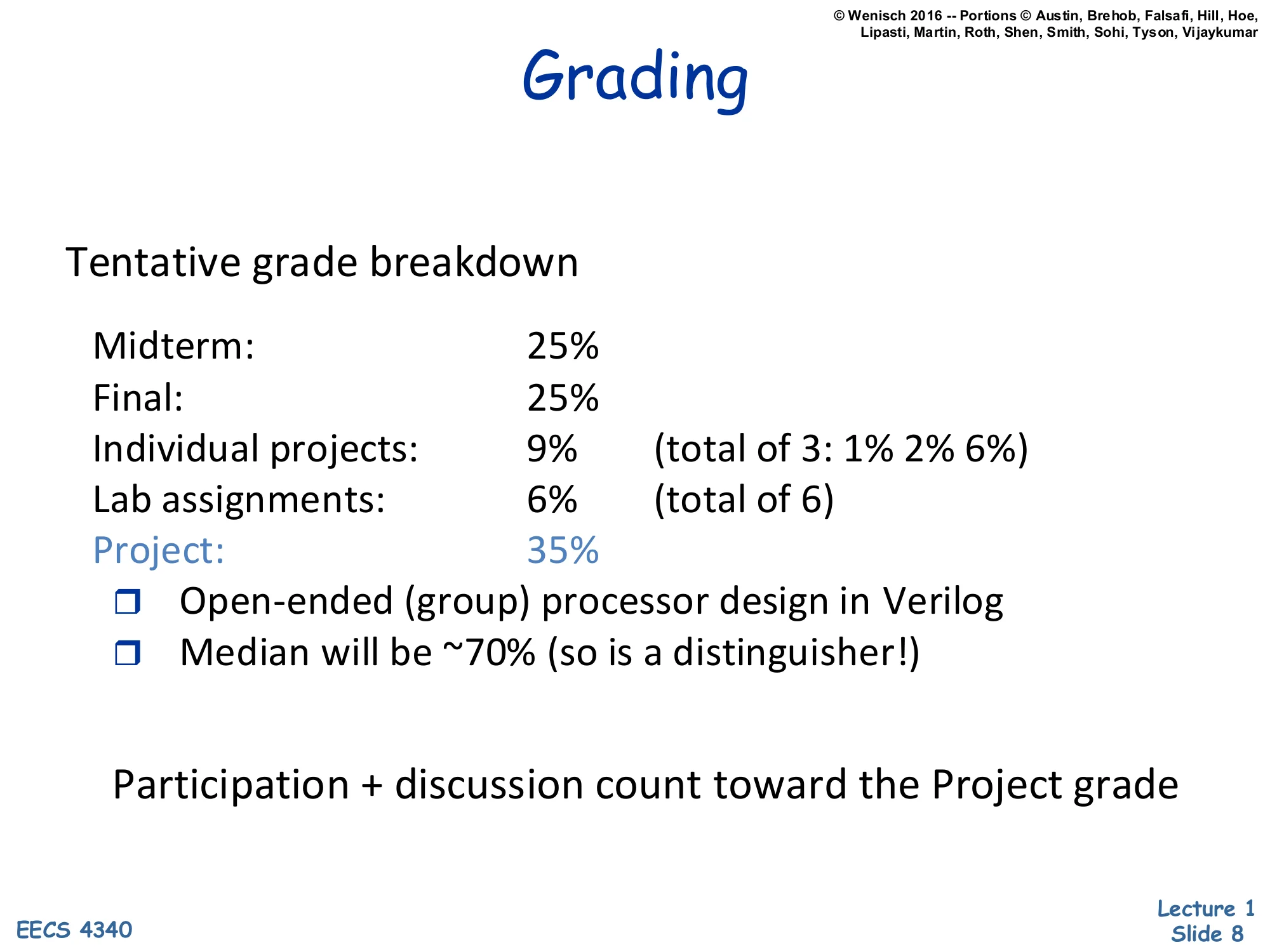
Tentative grade breakdown
| Component | Weight | Notes |
|---|---|---|
| Midterm | 25% | |
| Final | 25% | |
| Individual projects | 9% | (total of 3: 1% 2% 6%) |
| Lab assignments | 6% | (total of 6) |
| Project | 35% | Open-ended (group) processor design in Verilog. Median will be ~70% (so is a distinguisher!) |
Participation + discussion count toward the Project grade
Grading breakdown. The two written exams (midterm, final) together weight only 50%; individual projects (9% across three escalating projects worth 1/2/6%) and lab assignments (6% across six labs) cover the small-but-broad practice work. The remaining 35% is the open-ended group Verilog project — explicitly the highest-leverage component and the only one with a distinguisher dynamic (median target ~70%, so heavy compression at the top). Class participation and discussion roll into the project grade rather than being separately weighted, encouraging engagement during architecture critiques without requiring a separate participation rubric.
Grading (Cont.)
Show slide text
Grading (Cont.)
No late submissions, no kidding
Group studies are encouraged
Group discussions are encouraged
All lab assignments & individual projects must be the results of individual work
There is no tolerance for academic dishonesty. Please refer to the University Policy on cheating and plagiarism. Discussion and group studies are encouraged, but all submitted material must be the student’s individual work (or in the case of the project, individual group work).
Academic-integrity boilerplate with two important pragmatic rules. First, no late submissions — explicitly emphasized (“no kidding”), so students should plan toolchain/server problems to leave slack. Second, collaboration scope is bounded: you may discuss and study together, but lab assignments and individual projects must be each student’s individual work; only the open-ended Verilog project is a true group deliverable.
Hours (and hours) of work
Show slide text
Hours (and hours) of work
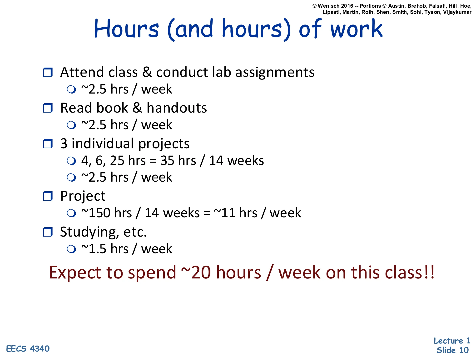
- Attend class & conduct lab assignments
- ~2.5 hrs / week
- Read book & handouts
- ~2.5 hrs / week
- 3 individual projects
- 4, 6, 25 hrs = 35 hrs / 14 weeks
- ~2.5 hrs / week
- Project
- ~150 hrs / 14 weeks = ~11 hrs / week
- Studying, etc.
- ~1.5 hrs / week
Expect to spend ~20 hours / week on this class!!
Time-budget reality check. Class+lab is 2.5 h/week, reading another 2.5 h/week, three escalating individual projects (4 + 6 + 25 hours, average ~2.5 h/week over 14 weeks), and the dominant group project at ~11 hours/week (150 hours total). Plus 1.5 hours of generic studying. Sum: ~20 hours/week, which is the canonical “4-credit graduate course” load and is roughly twice typical undergraduate expectations. The slide’s purpose is to set expectations before drop/add so students who can’t commit drop early.
Trends in computer hardware
A Paradigm Shift In Computing
Show slide text
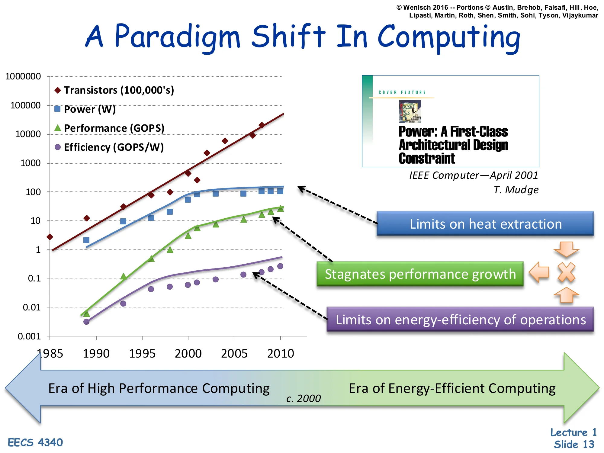
A Paradigm Shift In Computing
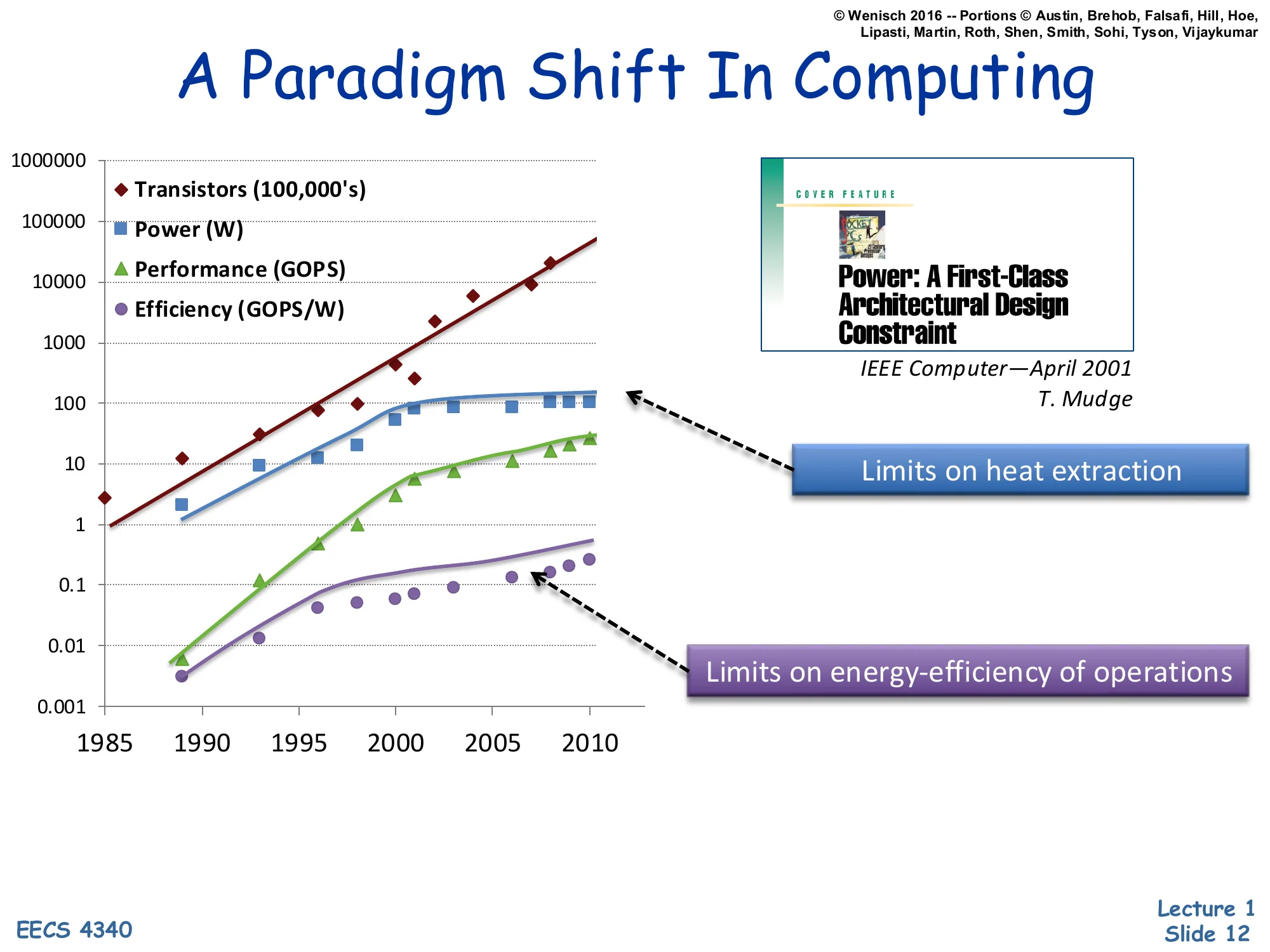
Log-scale plot, 1985–2010, of:
- Transistors (100,000’s) — rises ~5 orders of magnitude
- Power (W) — rises and plateaus around 100 W
- Performance (GOPS) — rises and bends down past ~2000
- Efficiency (GOPS/W) — rises and bends down past ~2000
Power: A First-Class Architectural Design Constraint — IEEE Computer, April 2001, T. Mudge
- Power plateau labeled: Limits on heat extraction
- Efficiency plateau labeled: Limits on energy-efficiency of operations
T. Mudge’s 2001 IEEE Computer paper “Power: A First-Class Architectural Design Constraint,” reproduced as a log-scale plot of four metrics from 1985 to 2010, makes the case that the old growth model broke around 2001–2005. Transistor count keeps climbing exponentially (Moore’s-Law-style — about 5 decades over 25 years), but power per chip plateaus near 100 W because of heat-extraction limits (you can’t pull more heat through a package without exotic cooling), and energy efficiency in GOPS/W plateaus because each operation’s voltage swing × capacitance can no longer shrink as fast as before. With both of those flat, raw Moore’s-Law transistor scaling can no longer be cashed out as proportional single-threaded performance growth. This single chart motivates the rest of the lecture: why we abandoned ever-faster single cores and pivoted to multicore plus DVFS.
A Paradigm Shift In Computing (annotated)
Show slide text
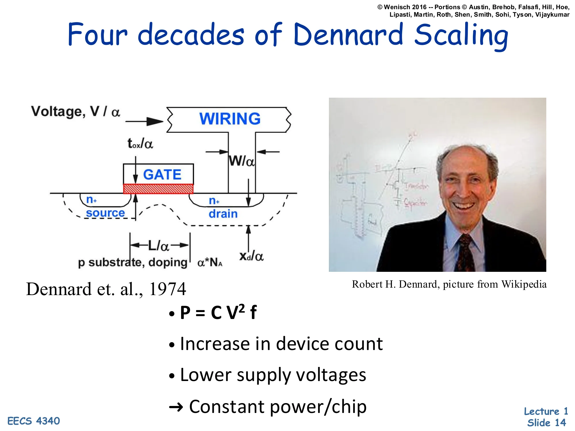
A Paradigm Shift In Computing
Same 1985–2010 chart, with extra annotations:
- Limits on heat extraction points at the power plateau
- Stagnates performance growth points at the performance bend
- Limits on energy-efficiency of operations points at the efficiency plateau
Bottom timeline arrow:
- Era of High Performance Computing → c. 2000 → Era of Energy-Efficient Computing
Annotated version of the previous chart. The new arrow at the bottom names the two eras: pre-2000 “High Performance Computing” when frequency and IPC scaled together so single-thread performance roughly doubled every ~18 months, and post-2000 “Energy-Efficient Computing” when the performance curve bends down because the power plateau forces architects to optimize joules-per-instruction, not just instructions-per-second. The third callout, stagnates performance growth, makes explicit the causal chain: heat-extraction limits cap power → frequency scaling stalls → single-thread performance flattens. Everything EECS 4340 covers later — multicore, DVFS, aggressive speculation, deeper memory hierarchies — is a response to this regime change.
Four decades of Dennard Scaling
Show slide text
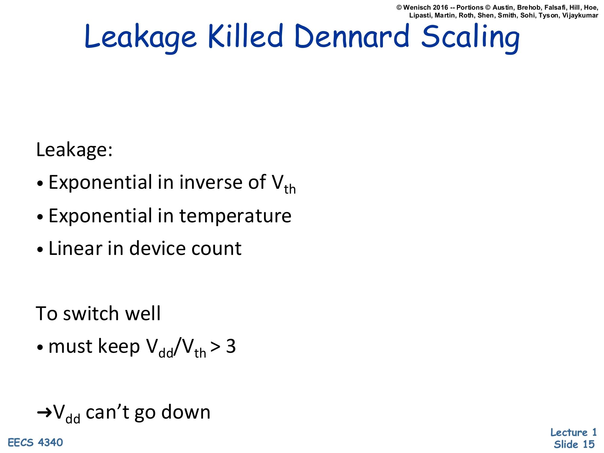
Four decades of Dennard Scaling
Diagram: MOSFET cross-section with scaling factors
- Voltage, V/α
- Wiring width W/α
- Oxide thickness tox/α
- Gate length L/α
- Source/drain depth xd/α
- p-substrate doping scales as α⋅NA
Dennard et al., 1974
- P=CV2f
- Increase in device count
- Lower supply voltages
- → Constant power/chip
The classic Dennard scaling picture from Dennard et al., 1974. If you shrink every linear dimension of a MOSFET — gate length L, wire width W, oxide thickness tox, junction depth xd — by a factor α, and you scale the supply voltage V by the same factor α (while increasing doping NA by α to preserve threshold behavior), then several things happen at once. Capacitance C scales as 1/α, frequency f scales as α, and switching power per transistor P=CV2f scales as 1/α2⋅1/α=1/α3 for capacitance, voltage-squared, and timing — but if you also pack α2 more transistors into the same chip area, the per-chip power stays roughly constant. The slide’s punchline — constant power/chip — is the magical property that powered four decades of “free” performance: every process node delivered more, faster transistors at the same thermal budget. The next slide explains why this magic stopped.
Leakage Killed Dennard Scaling
Show slide text
Leakage Killed Dennard Scaling
Leakage:
- Exponential in inverse of Vth
- Exponential in temperature
- Linear in device count
To switch well
- must keep Vdd/Vth>3
→ Vdd can’t go down
Why Dennard scaling broke. Static leakage current through an “off” transistor grows exponentially as the threshold voltage Vth shrinks (because subthreshold leakage scales as roughly exp(−Vth/kT)), grows exponentially with temperature, and grows linearly with device count. To keep gates fast and noise-immune you need Vdd/Vth≳3, which means lowering Vdd requires also lowering Vth — but lower Vth explodes leakage power. The combined constraint pins Vdd near ~1 V from the early 2000s onward. With Vdd frozen, the V2 in P=CV2f no longer shrinks, so per-transistor switching power stops dropping, and packing α2 more transistors per chip now linearly increases chip power instead of staying flat. That is the death of Dennard scaling and the direct cause of the dark-silicon problem and the multicore pivot.
Multicore: Solution to Power-constrained design?
Show slide text
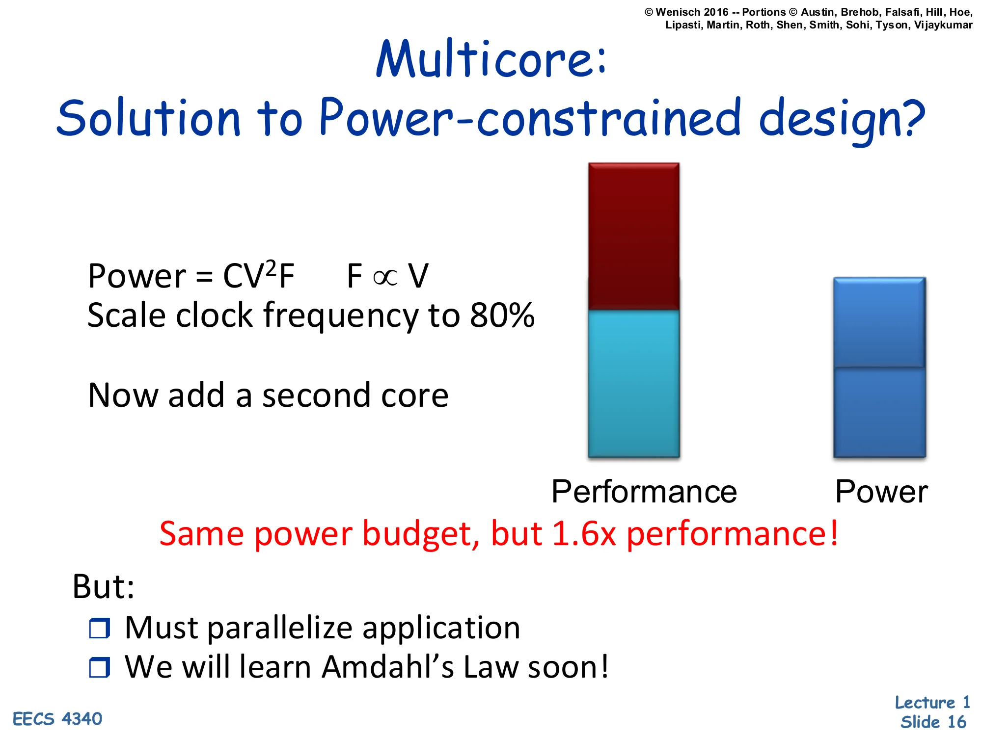
Multicore: Solution to Power-constrained design?
P=CV2FF∝V
Scale clock frequency to 80%
Now add a second core
Bar chart: Performance bar (red on top of teal) vs. Power bar (one half-bar tall) — “Same power budget, but 1.6× performance!”
But:
- Must parallelize application
- We will learn Amdahl’s Law soon!
The textbook multicore argument. Dynamic power is P=CV2F and, in the regime where you must lower voltage to lower frequency, F∝V, so P∝F3. Drop the clock to 80% of its original frequency: power drops to 0.83≈0.51 — about half. Now spend the recovered ~50% of your power budget on a second identical core also clocked at 80%. The two-core chip uses 2×0.51≈1.02 of the original single-core power (essentially the same budget) while delivering up to 2×0.8=1.6× the throughput on parallel work. This is why every chip after ~2005 went multicore. The catch, flagged at the bottom: throughput only materializes if the application can actually be parallelized, which is bounded by Amdahl’s Law — the lecture’s next major topic. DVFS generalizes this trick by adjusting voltage and frequency at runtime.
Memory Wall
Show slide text
Memory Wall
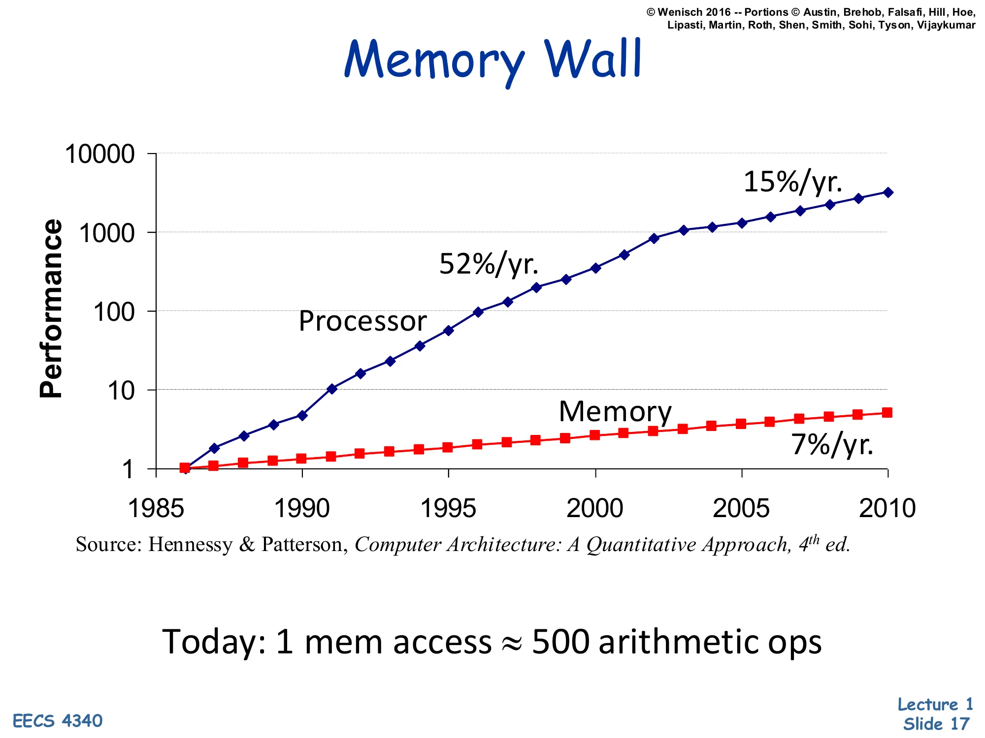
Log-scale performance vs. year (1985–2010):
- Processor: 52%/yr. through ~2003, then 15%/yr.
- Memory: 7%/yr. throughout
Source: Hennessy & Patterson, Computer Architecture: A Quantitative Approach, 4th ed.
Today: 1 mem access ≈ 500 arithmetic ops
The memory wall chart, from H&P 4th edition. Processor performance grew 52%/year from 1986 through ~2003 (the Dennard/frequency era), then slowed to 15%/year as the multicore/IPC era took over. Main-memory access time only improved ~7%/year for the entire window. The compounding gap means a single off-chip DRAM access today costs roughly 500 arithmetic operations of opportunity cost. This single number drives the rest of the memory-hierarchy curriculum: aggressive caches, hardware prefetching, deep store buffers, out-of-order execution to overlap misses, and (in modern systems) hardware-managed TLBs and large LLCs. Without those, a CPU would spend the vast majority of cycles waiting on memory.
Reliability Wall
Show slide text
Reliability Wall
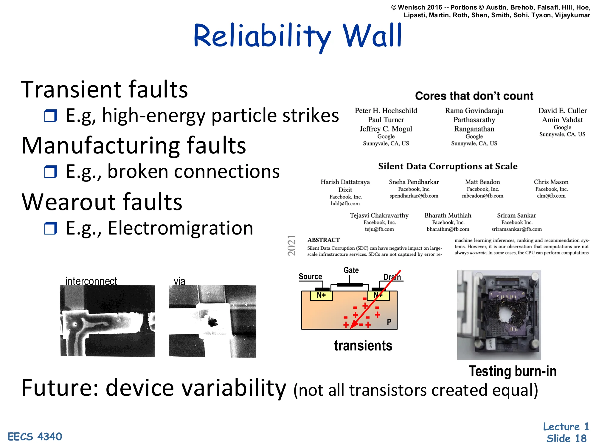
Transient faults
- E.g., high-energy particle strikes
Manufacturing faults
- E.g., broken connections
Wearout faults
- E.g., Electromigration
Referenced article: Cores that don’t count / Silent Data Corruptions at Scale (2021), with authors from Google and Sunnyvale.
Images: interconnect/via micrograph, transient-fault MOSFET diagram (Source/Gate/Drain with particle strike), “Testing burn-in”.
Future: device variability (not all transistors created equal)
The reliability wall: as transistors shrink, three classes of faults become first-class architectural concerns. Transient faults are one-time bit flips caused by high-energy cosmic rays or alpha particles striking storage cells; smaller cells store fewer charges so are easier to flip. Manufacturing faults are permanent defects from lithography variation, and wearout faults like electromigration accumulate over a chip’s lifetime and eventually break interconnects. The cited 2021 industry papers (“Cores that don’t count,” “Silent Data Corruptions at Scale”) from Google show that fleet-scale deployments now see individual cores silently producing wrong arithmetic results — not crashes, not parity errors, just quiet computational corruption. The closing point — device variability, not all transistors created equal — is the core thesis: at modern process nodes, two transistors patterned identically perform measurably differently, so future architectures must assume hardware is statistically unreliable.
Renaissance of Comp. Arch. Research
Show slide text
Renaissance of Comp. Arch. Research
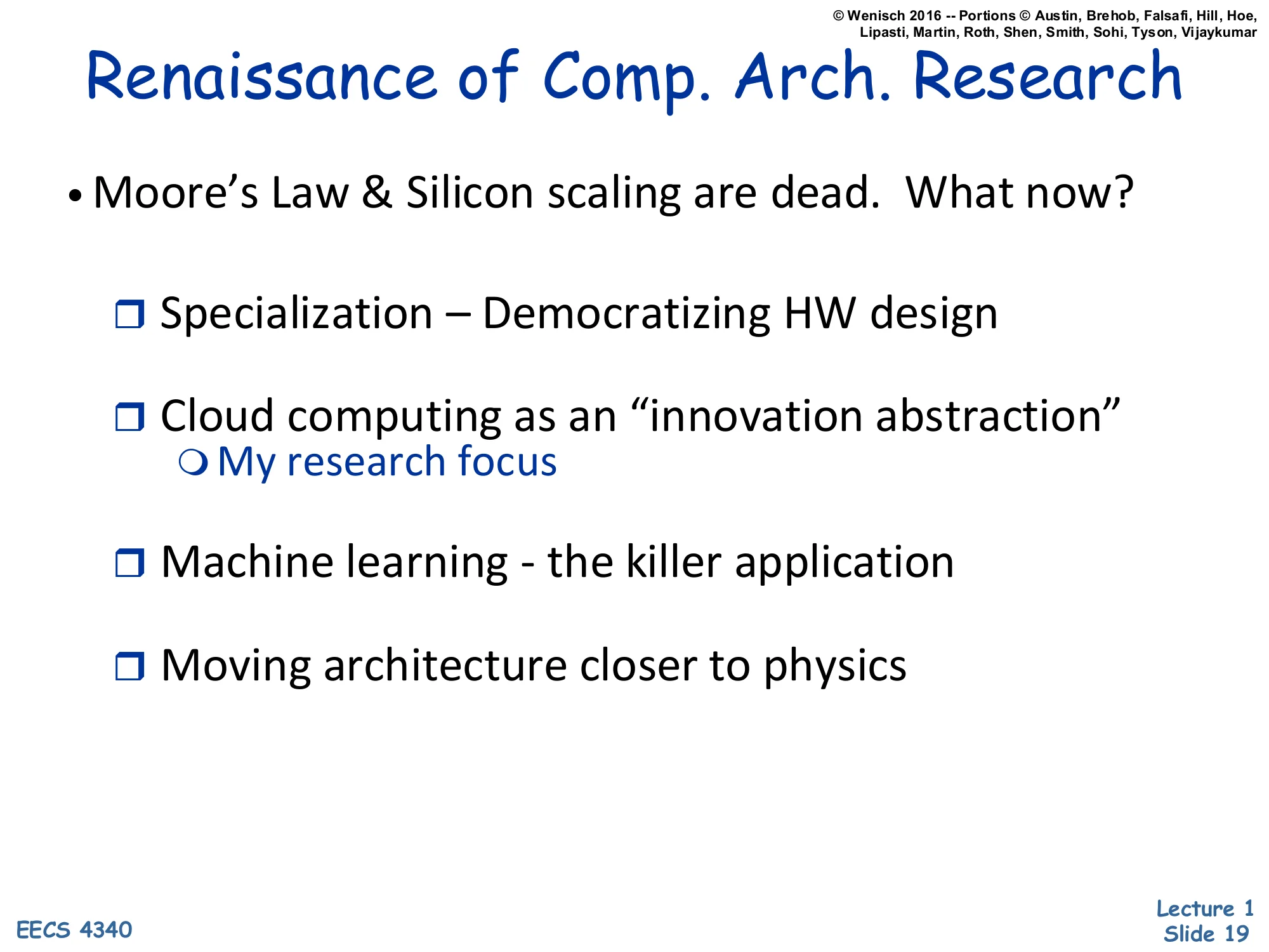
Moore’s Law & Silicon scaling are dead. What now?
- Specialization — Democratizing HW design
- Cloud computing as an “innovation abstraction”
- My research focus
- Machine learning - the killer application
- Moving architecture closer to physics
Khan’s pitch for why now is an exciting time to study architecture. With Moore’s Law and silicon scaling effectively dead, four research directions have opened up. Specialization (domain-specific accelerators, open ISAs like RISC-V, chiplets) is democratizing hardware design so smaller teams can ship custom silicon. Cloud computing as an innovation abstraction — Khan’s own area — treats the datacenter as the new design target where one good microarchitectural improvement is amortized across millions of servers. Machine learning is the workload that finally makes specialization pay off at scale (TPUs, GPUs, NPUs). Moving architecture closer to physics points at near-memory compute, optical interconnects, and analog/neuromorphic devices. The slide frames the rest of the course’s classical out-of-order/cache content as the foundation you need before you can responsibly innovate in any of these directions.
Fundamental concepts
Five key principles to performance
Show slide text
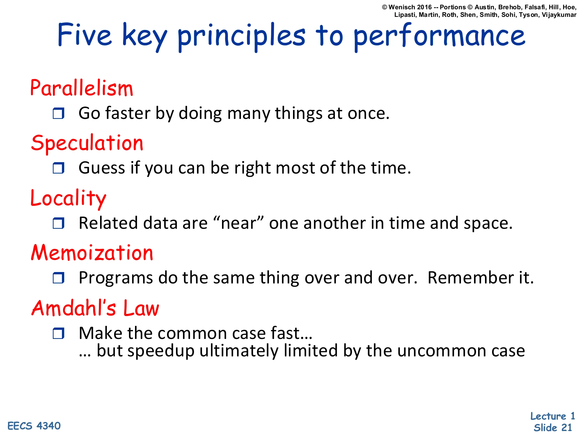
Five key principles to performance
Parallelism
- Go faster by doing many things at once.
Speculation
- Guess if you can be right most of the time.
Locality
- Related data are “near” one another in time and space.
Memoization
- Programs do the same thing over and over. Remember it.
Amdahl’s Law
- Make the common case fast… …but speedup ultimately limited by the uncommon case
Khan’s mental model for the rest of the course: every architectural technique you’ll see is a specific instance of one of five principles. Parallelism — pipelining, superscalar issue, multicore, SIMD — exploits independent work. Speculation — branch prediction, speculative execution, value prediction — bets on the common-case answer to hide latency. Locality — caches, TLBs, register allocation — exploits the fact that recent and nearby data are likely to be reused. Memoization — branch predictors as cached outcomes, trace caches, micro-op caches — saves the result of expensive computations to skip them next time. Amdahl’s Law — the meta-principle that optimizing the common case is great but the un-optimized fraction eventually dominates total runtime. These five principles are referenced explicitly throughout the lecture series, so a student who internalizes them now has a vocabulary for every later technique.
Parallelism: Work and Critical Path
Show slide text
Parallelism: Work and Critical Path
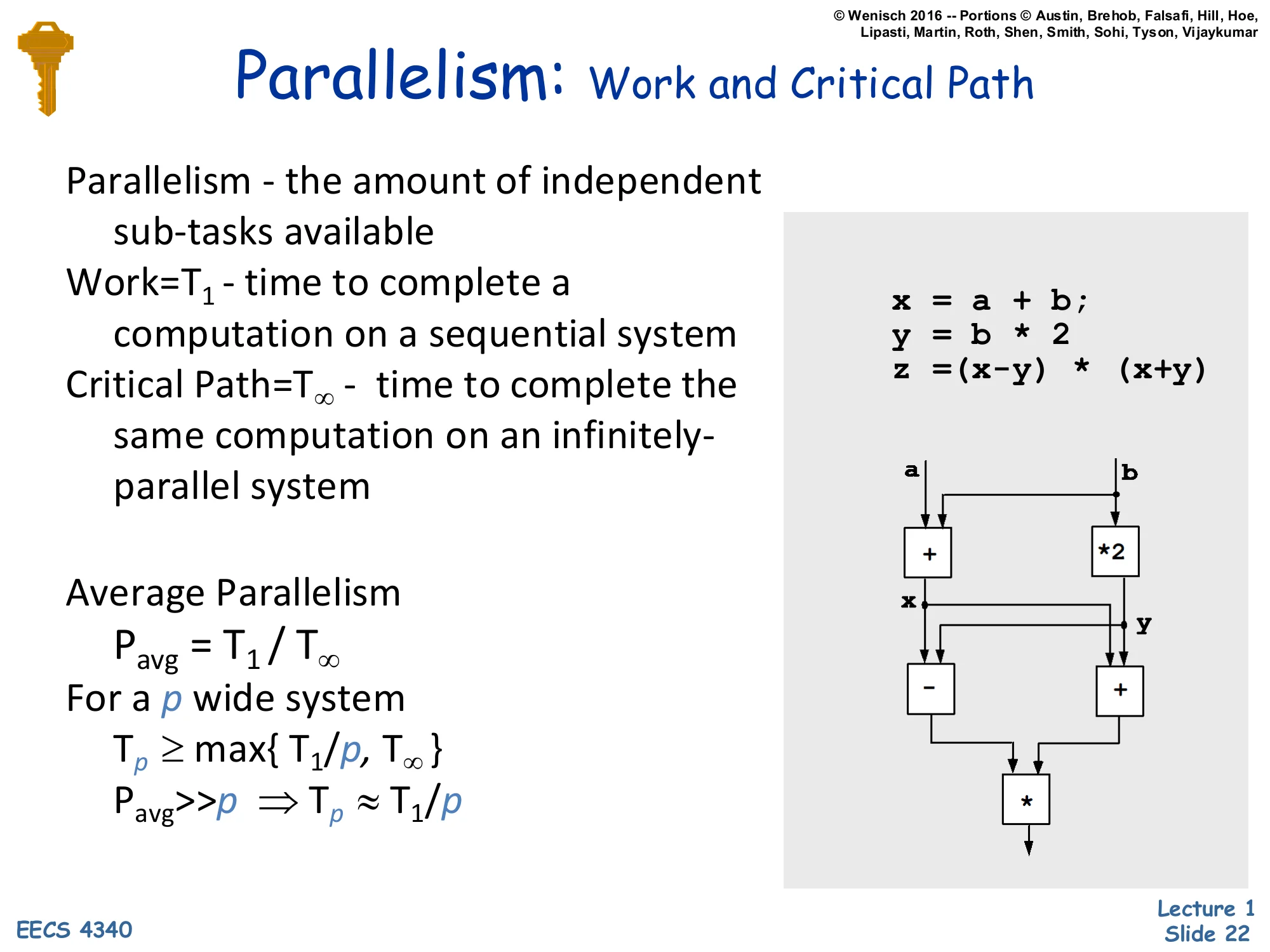
Parallelism — the amount of independent sub-tasks available
Work = T1 — time to complete a computation on a sequential system
Critical Path = T∞ — time to complete the same computation on an infinitely-parallel system
Average Parallelism
Pavg=T1/T∞
For a p wide system
Tp≥max{T1/p,T∞}
Pavg≫p⇒Tp≈T1/p
Example code:
x = a + b;y = b * 2z = (x - y) * (x + y)Dataflow graph: a,b → + and b → *2, then x,y → - and x,y → +, then → * (final result).
Formal vocabulary for work and critical path from parallel-algorithm theory. Work T1 is wall-clock time on a single processor; critical path T∞ is wall-clock time given infinitely many processors and zero communication cost. Their ratio Pavg=T1/T∞ is the average parallelism — how many processors you could keep busy on average. For a finite p-wide machine, Tp≥max{T1/p,T∞}: you’re bounded both by total work spread across p workers and by the critical path. When Pavg≫p, work dominates and you get near-linear speedup (Tp≈T1/p); when p approaches Pavg, the critical path takes over and adding cores stops helping. The example computes z=(x−y)(x+y) where x=a+b and y=2b. Sequentially that’s 4 ops (work = 4); in parallel the dataflow graph has depth 3 — the + and ∗2 run in parallel at level 1, then − and + at level 2, then the final ∗ at level 3 — so T∞=3 and Pavg=4/3. Modest, but it illustrates that even small expressions have measurable parallelism if you can extract it.
Amortization & Speculation
Show slide text
Amortization & Speculation
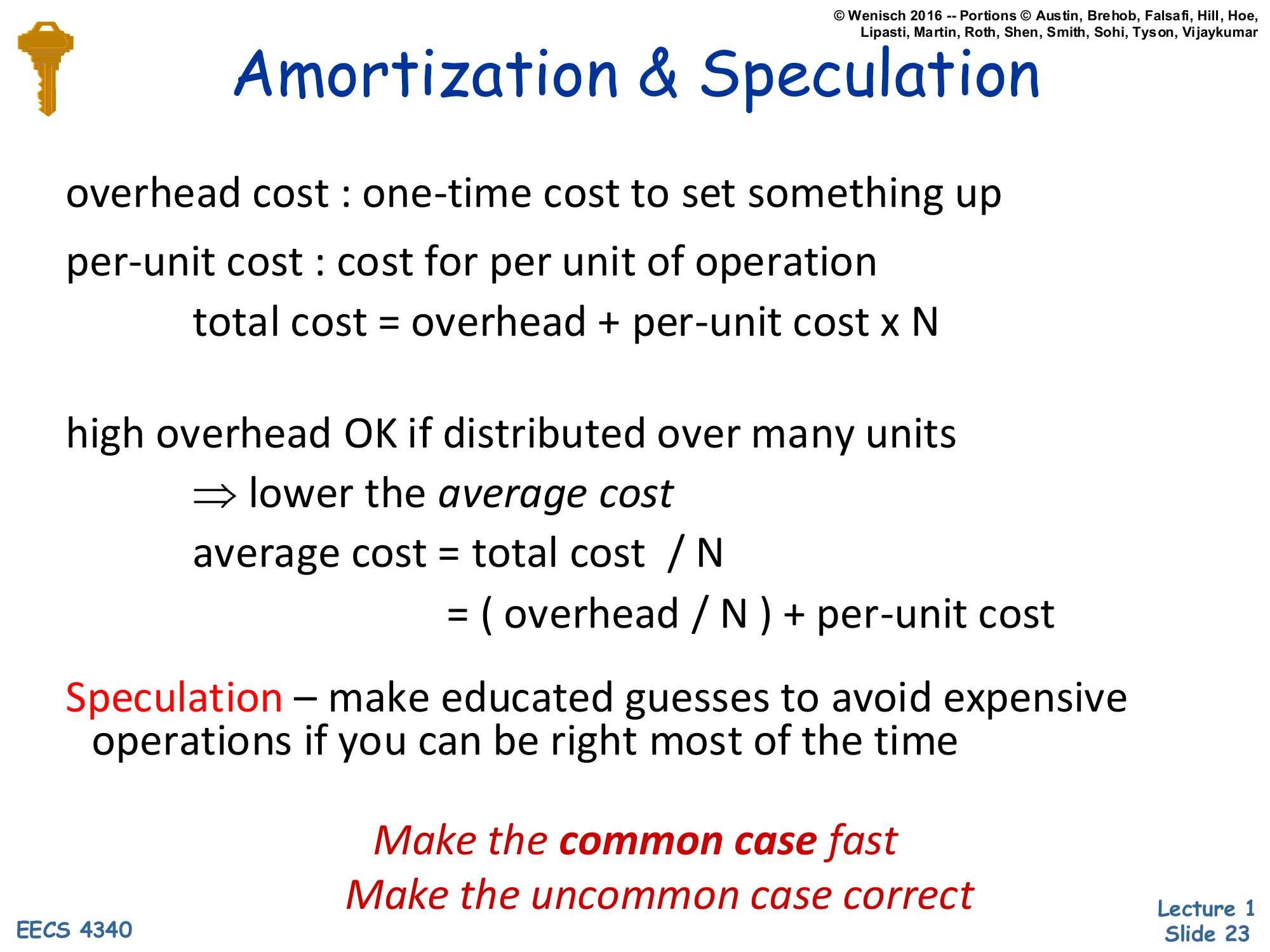
overhead cost: one-time cost to set something up
per-unit cost: cost for per unit of operation
total cost=overhead+per-unit cost×N
high overhead OK if distributed over many units
⇒ lower the average cost
average cost=total cost/N=(overhead/N)+per-unit cost
Speculation — make educated guesses to avoid expensive operations if you can be right most of the time
Make the common case fast
Make the uncommon case correct
Two related performance ideas. Amortization: if a technique has fixed overhead O and per-use cost c, total cost across N uses is O+cN and average cost is O/N+c, which approaches c as N grows. So a technique with high one-time cost (e.g., training a branch predictor, filling a cache line, building an indexed page table) is fine if it gets reused enough. This is why architecture is so concerned with hit rates and reuse distances. Speculation is the dual idea: take an expensive-to-resolve operation (a branch, a load whose address depends on an unfinished store) and guess the answer immediately. If you guess right most of the time you avoid the wait; if you guess wrong you must roll back. The two slogans at the bottom — make the common case fast, make the uncommon case correct — are the design discipline for any speculative mechanism: optimize for the prediction-hit path, and reserve a (slower) recovery path for the rare miss.
Locality Principle
Show slide text
Locality Principle
One’s recent past is a good indication of near future.
- Temporal Locality: If you looked something up, it is very likely that you will look it up again soon
- Spatial Locality: If you looked something up, it is very likely you will look up something nearby next
Locality == Patterns == Predictability
Converse: Anti-locality: If you haven’t done something for a very long time, it is very likely you won’t do it in the near future either
The two flavors of locality. Temporal locality: if a program just touched address A, it is likely to touch A again soon — so worth caching. Spatial locality: if it touched address A, it is likely to touch A+δ for small δ — so worth fetching adjacent bytes proactively (this is why a cache line is 64 bytes, not 1). Khan’s slogan locality == patterns == predictability is the meta-claim that locality is the property that makes hardware speedups possible — without patterns, every memory access is a coin flip and no architectural cleverness can help. The anti-locality corollary motivates eviction policies: things untouched for a long time are unlikely to be touched soon, so LRU is a reasonable eviction strategy. Locality directly supports caches, TLBs, prefetchers, and even the working-set theory underlying virtual memory.
Memoization
Show slide text
Memoization
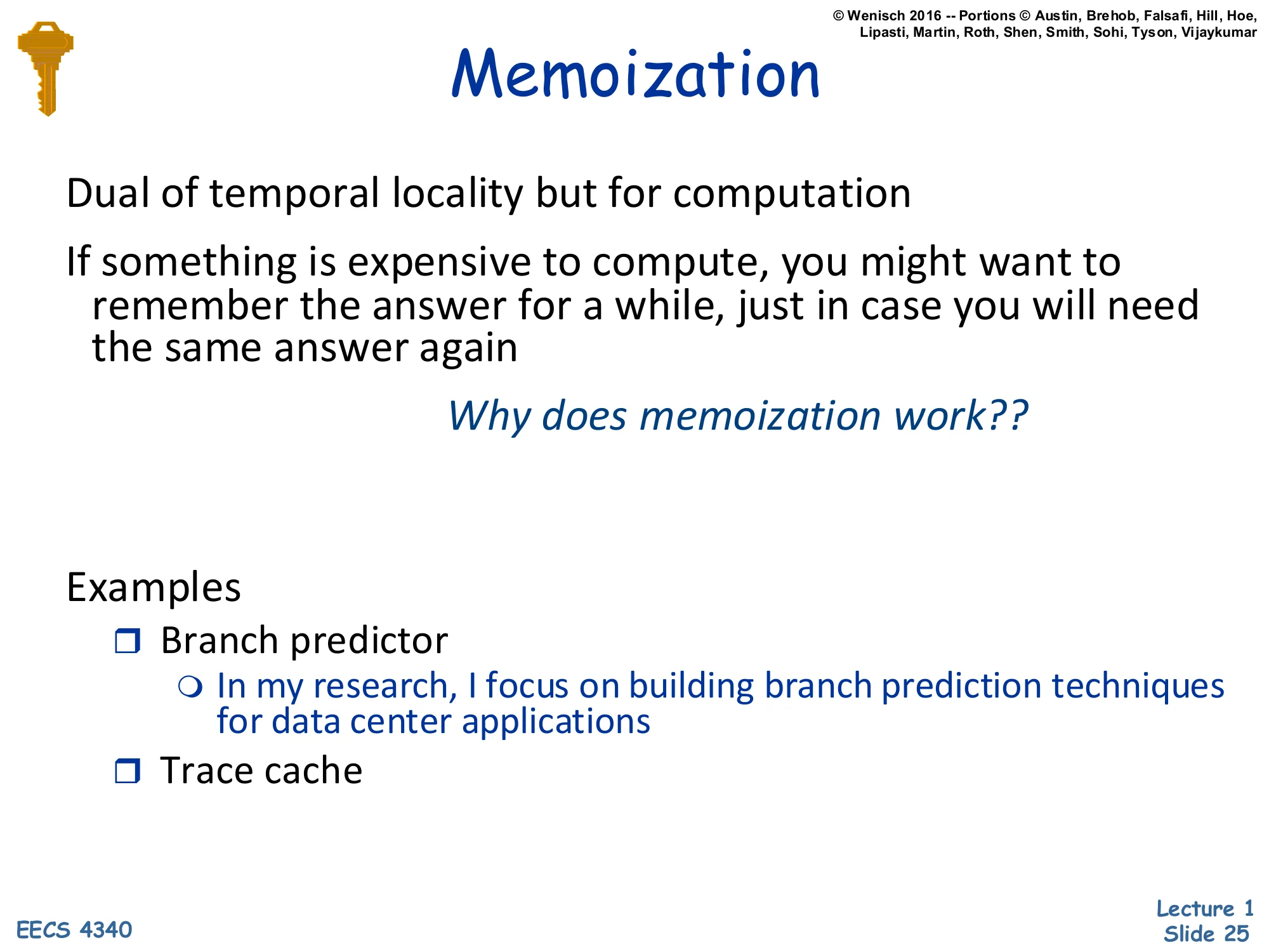
Dual of temporal locality but for computation
If something is expensive to compute, you might want to remember the answer for a while, just in case you will need the same answer again
Why does memoization work??
Examples
- Branch predictor
- In my research, I focus on building branch prediction techniques for data center applications
- Trace cache
Memoization in hardware. While temporal locality caches data you’ve recently accessed, memoization caches the result of a computation you’ve recently performed. The two examples on the slide make it concrete. A branch predictor is a memoization table for the function “will this branch PC be taken?” — past outcomes are stored in a BHT of saturating counters and looked up on the next encounter. Khan notes that his own research builds branch prediction techniques targeted at datacenter workloads, where the working set of branches far exceeds typical predictor capacity. A trace cache memoizes a decoded sequence of instructions following a particular control-flow path; rather than re-fetching and re-decoding, the CPU reads the trace and replays it. Why memoization works is the same answer as why caches work: program behavior is highly repetitive, so storing recent answers pays off across many future identical queries.
Amdahl's Law
Show slide text
Amdahl’s Law
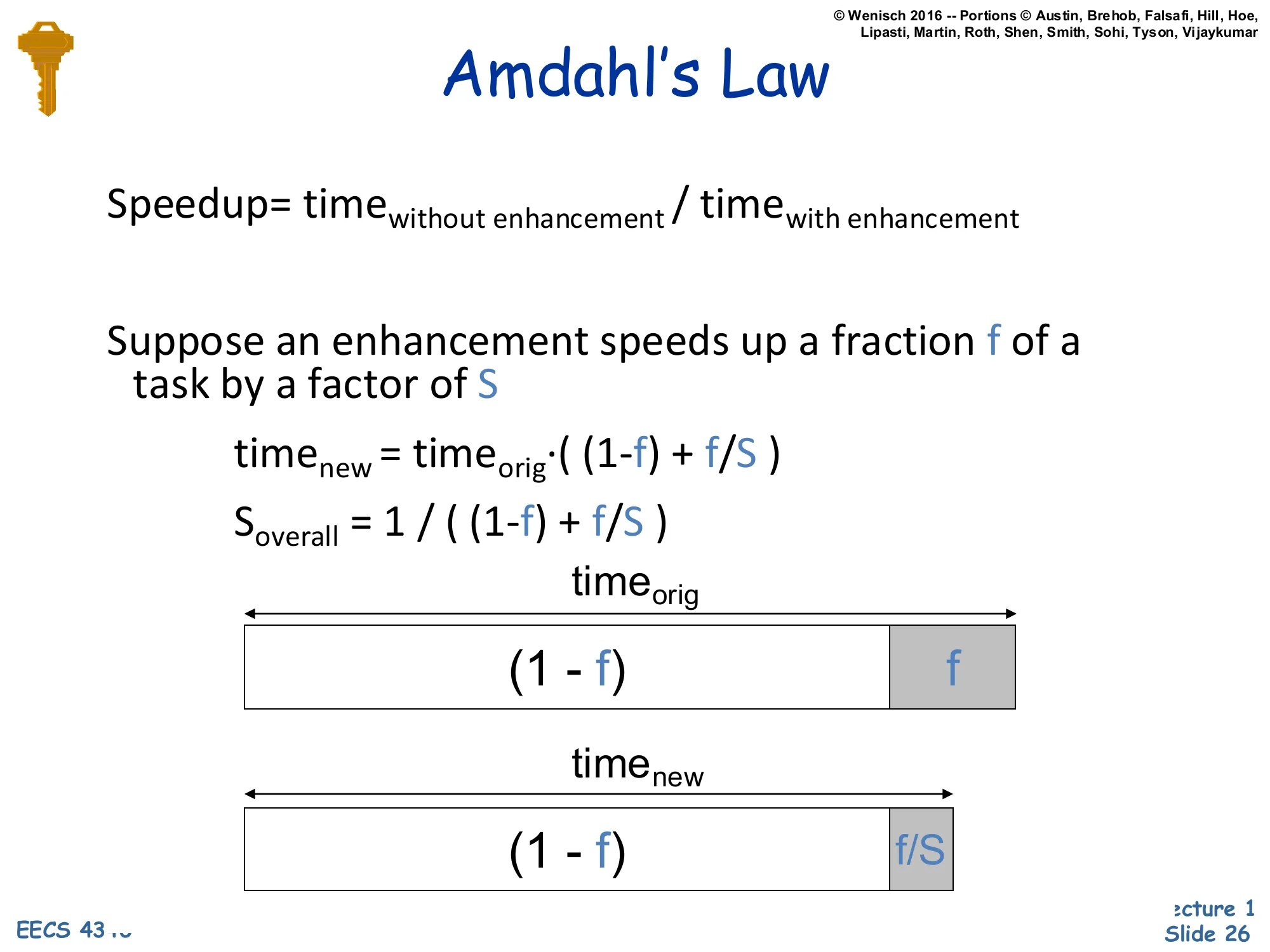
Speedup=timewith enhancementtimewithout enhancement
Suppose an enhancement speeds up a fraction f of a task by a factor of S
timenew=timeorig⋅((1−f)+f/S)
Soverall=(1−f)+f/S1
Diagram: timeorig split into two segments — a (1−f) block (un-enhanced) and an f block (enhanced). timenew has the same (1−f) block but the enhanced part shrinks to f/S.
The formal statement of Amdahl’s Law. Define speedup as Soverall=Torig/Tnew. If an enhancement covers a fraction f of original execution time and runs that fraction S× faster, then Tnew=Torig((1−f)+f/S)⟹Soverall=(1−f)+f/S1. The diagram shows why: only the f-fraction shrinks (to f/S); the (1−f) part is unchanged. Two consequences worth memorizing. First, even for S→∞, the speedup is capped at 1/(1−f) — so a 90%-parallelizable program (f=0.9) maxes out at 10× no matter how many cores you throw at it. Second, modest enhancements applied to large fractions beat huge enhancements applied to tiny fractions. This is the formal version of the make-the-common-case-fast slogan and is the single most-cited result in computer architecture; you’ll see it again when reasoning about CPI components, AMAT miss penalties, and parallel speedup curves.
Readings
Show slide text
Readings
For this week:
- The electronic copy of H&P (5th ed.) is available online for free by Columbia University Libraries,
- H&P Chapter 1, Appendix A
Reading assignment: Hennessy & Patterson, Computer Architecture: A Quantitative Approach, 5th edition, Chapter 1 (fundamentals of quantitative design and analysis — covers the same iron-law and Amdahl’s-Law material at greater depth) and Appendix A (review of pipelining, the prerequisite for L03). Columbia students access it for free through CLIO.
Announcements

Show slide text
Announcements
Labs start next Wednesday
- Please bring your computer
- Involve graded assignments
- Attendance is required and graded
Project #1
- Will be released before Monday (26-Jan-26)
- Due 4-Feb-26
- More details in the lab next week
End-of-lecture logistics. Labs start the following Wednesday — students must bring their own laptop, the labs are graded, and attendance counts. Project #1 (the smallest of the three individual projects, weighted 1%) will be released before Monday Jan 26, 2026, with a due date of Feb 4, 2026 — about a 9-day window. Details will be walked through in the next lab session.