L12 · Caches

L12 · Caches

Topic: memory · 41 pages

EECS 4340 Lecture 12 — Basic Caches

Slide 1

Announcements

Slide 2

Show slide text

Announcements

• Project #4
  • Due: 22-April-26
• Project meetings
  • Mondays and Wednesdays during my office hours

https://courseworks2.columbia.edu/courses/237081

Readings

Slide 3

Show slide text

Readings

For today:

• H & P Chapter 2.1, Appendix B.1, and B.2

For Wednesday:

• H & P Chapter 2.2, 2.3, and Appendix B.3
• Improving direct-mapped cache performance by the addition of a small fully-associative cache and prefetch buffers, https://dl.acm.org/doi/abs/10.1145/325096.325162

Recap: Branch Prediction

Slide 4

BP Implementation Challenges

Slide 5

Show slide text

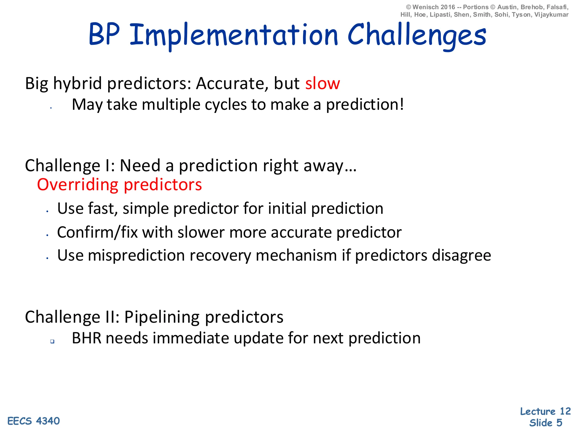
BP Implementation Challenges

Big hybrid predictors: Accurate, but slow

• May take multiple cycles to make a prediction!

Challenge I: Need a prediction right away…

• Overriding predictors
  • Use fast, simple predictor for initial prediction
  • Confirm/fix with slower more accurate predictor
  • Use misprediction recovery mechanism if predictors disagree

Challenge II: Pipelining predictors

• BHR needs immediate update for next prediction

Modern branch predictors face a frustrating tension: bigger, smarter, hybrid predictors achieve higher accuracy, but their lookup latency can stretch past a single fetch cycle — and the front end needs a direction every cycle to keep fetching. The lecture frames two implementation challenges. The first is producing a prediction in time. Overriding predictors solve this by running a fast, simple predictor (e.g. a small bimodal table) in parallel with a larger, slower one; the fast prediction steers fetch immediately, and the slow predictor either confirms it (no action) or contradicts it (a partial squash recovers and steers fetch with the better answer). The cost of an override is small compared to a full mispredict because no instructions have committed. The second challenge is pipelining the predictor itself: the global branch history register (BHR) used by correlating predictors like gshare needs to be updated speculatively the cycle a branch is predicted, so that the next branch’s prediction sees current history. Real designs maintain a checkpointed history that can be restored on a mispredict so the BHR snaps back to the architectural truth on recovery.

Mis-speculation Recovery

Slide 6

Show slide text

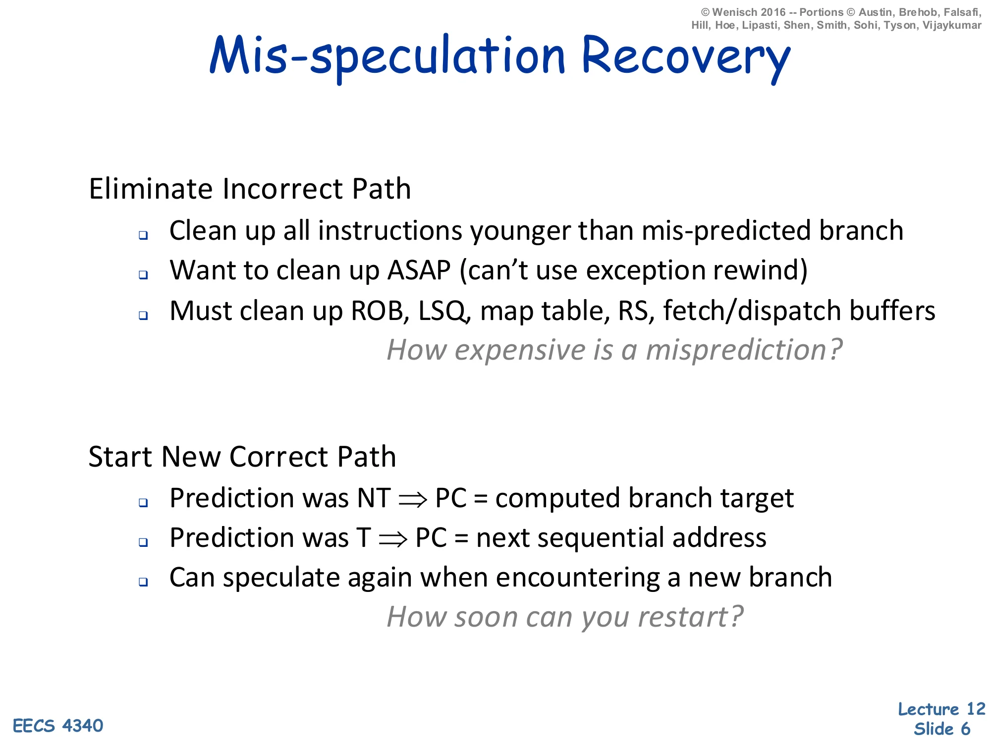
Mis-speculation Recovery

Eliminate Incorrect Path

• Clean up all instructions younger than mis-predicted branch
• Want to clean up ASAP (can’t use exception rewind)
• Must clean up ROB, LSQ, map table, RS, fetch/dispatch buffers

How expensive is a misprediction?

Start New Correct Path

• Prediction was NT $\Rightarrow$ PC = computed branch target
• Prediction was T $\Rightarrow$ PC = next sequential address
• Can speculate again when encountering a new branch

How soon can you restart?

When a branch is resolved as mispredicted, every younger instruction in the machine is on the wrong path and must be eliminated before it commits. The slide enumerates the structures that hold speculative state: the ROB, the load-store queue, the rename map table, reservation stations, and the fetch/dispatch buffers. Recovery cannot piggyback on the precise-exception rewind machinery because exceptions are rare and slow; mispredictions happen on roughly 5–10% of branches and must be handled in a couple of cycles to keep IPC up. Once the wrong-path instructions are gone, the front end is redirected: if the prediction was not-taken the corrected PC is the computed branch target; if it was taken the corrected PC is the fall-through (next sequential) address. After redirection the machine speculates anew on the next branch it encounters — there is no penalty for re-speculating immediately. The two cost questions on the slide motivate the fast branch recovery hardware on the next slide: faster recovery means fewer wasted cycles per mispredict, which directly reduces effective CPI.

Fast Branch Recovery

Slide 7

Show slide text

Fast Branch Recovery

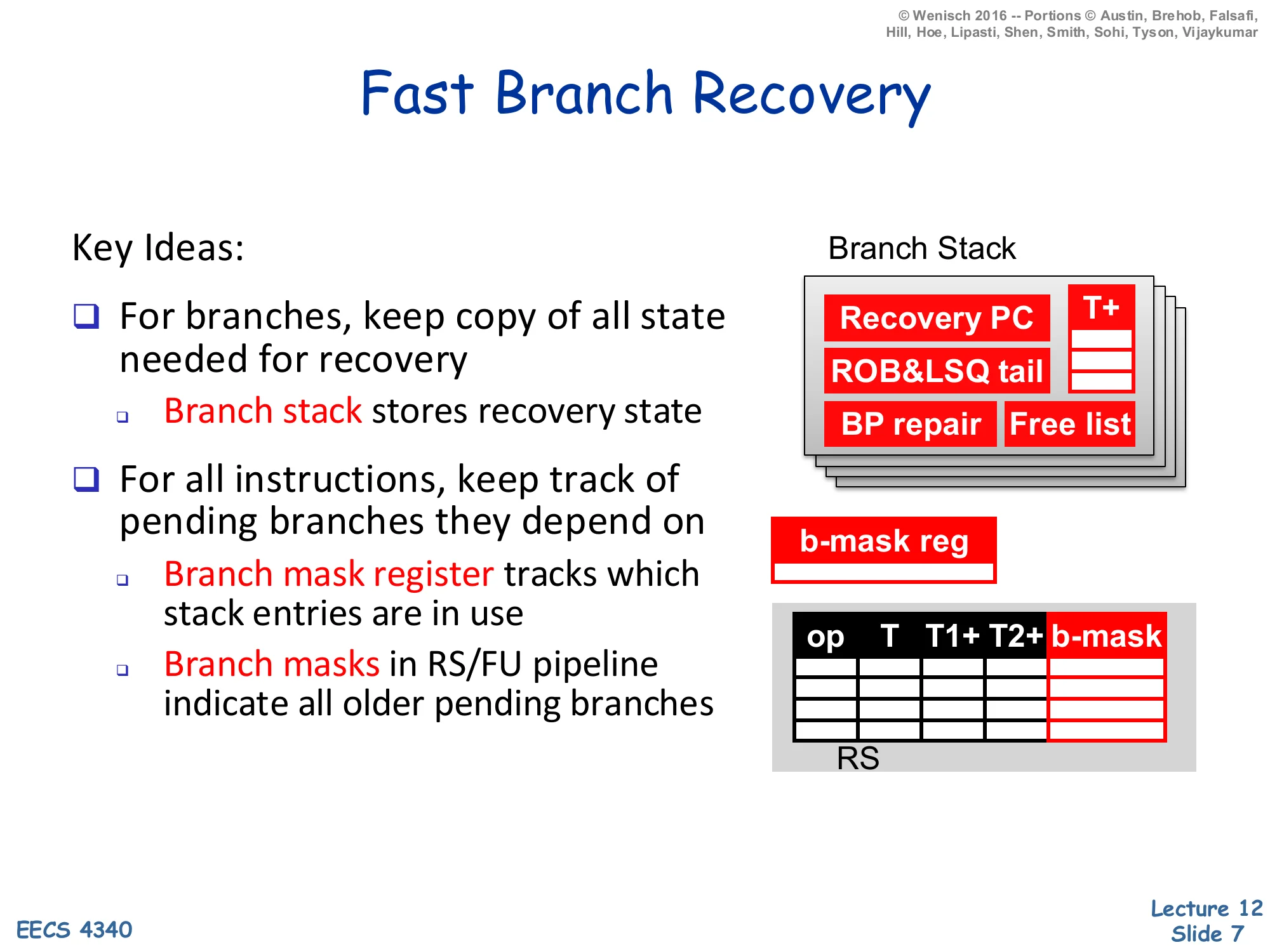
Key Ideas:

• For branches, keep copy of all state needed for recovery
  • Branch stack stores recovery state
• For all instructions, keep track of pending branches they depend on
  • Branch mask register tracks which stack entries are in use
  • Branch masks in RS/FU pipeline indicate all older pending branches

Branch Stack entries:

• Recovery PC, T+ (rename map snapshot)
• ROB & LSQ tail
• BP repair, Free list

RS columns: op, T, T1+, T2+, b-mask

Fast branch recovery makes mispredictions cheap by checkpointing the architectural state at every speculative branch instead of unwinding the ROB one entry at a time. Each branch pushes a Branch Stack entry holding everything the front end needs to resume on the correct path: the recovery PC (next-sequential or branch-target depending on prediction), a snapshot of the rename map and free list, the BHR/RAS state for the predictor (“BP repair”), and the ROB/LSQ tail pointers so younger entries can be invalidated en masse. A small branch-mask register tracks which Branch Stack entries are live. Every in-flight instruction carries a branch mask in its RS/FU pipeline payload that names which still-unresolved branches it depends on; when a branch resolves correctly its bit is cleared from every mask in one broadcast, and when it mispredicts every instruction whose mask has that bit set is squashed in a single cycle. Compare this to walking the ROB tail-pointer by tail-pointer: fast branch recovery turns an O(n) clean-up into an O(1) snapshot restore, which is what makes deep speculative machines tolerable.

Wide Instruction Fetch Issues

Slide 8

Show slide text

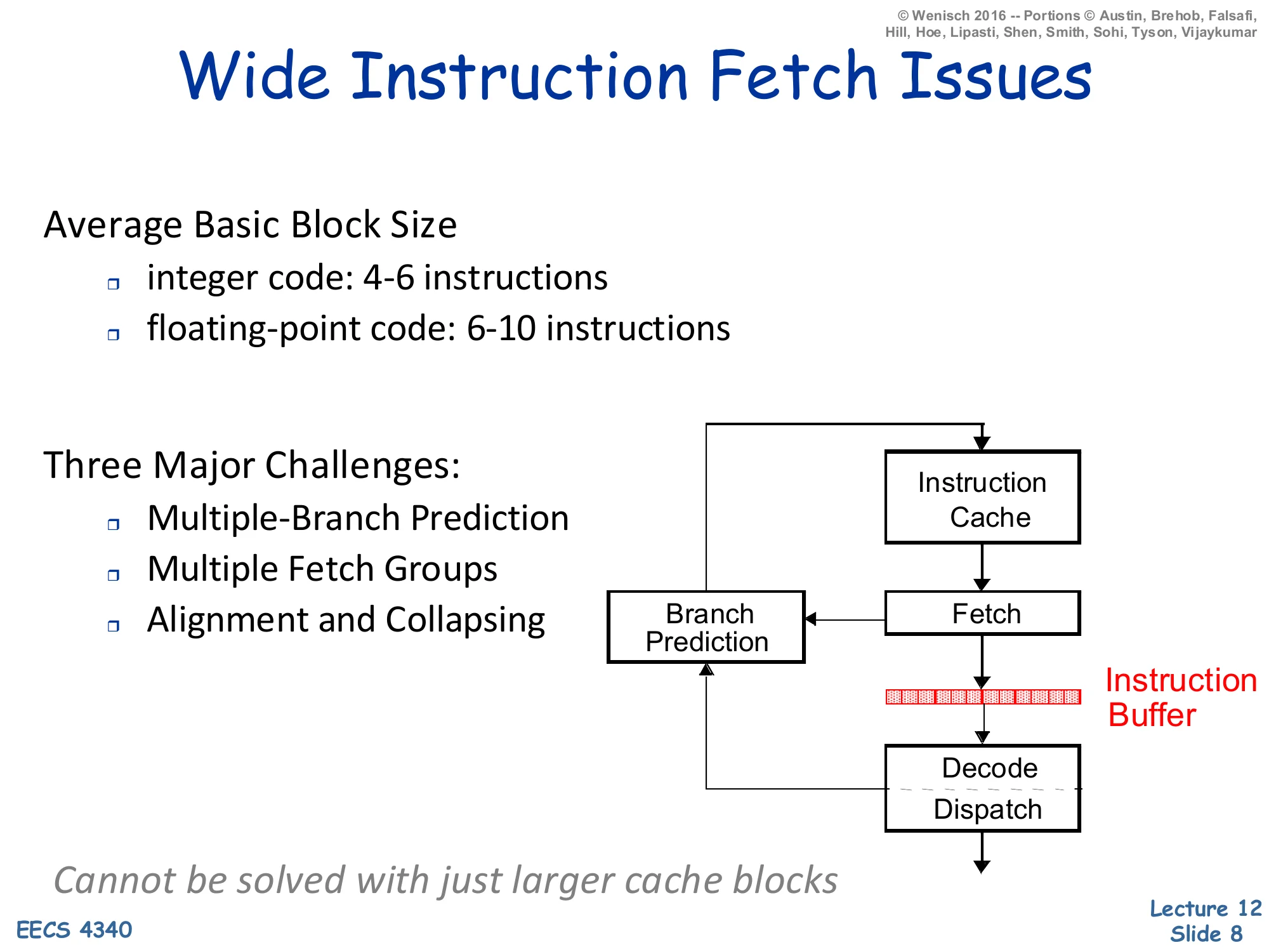
Wide Instruction Fetch Issues

Average Basic Block Size

• integer code: 4–6 instructions
• floating-point code: 6–10 instructions

Three Major Challenges:

• Multiple-Branch Prediction
• Multiple Fetch Groups
• Alignment and Collapsing

Pipeline: Instruction Cache → Fetch → Instruction Buffer → Decode/Dispatch, with Branch Prediction loop into Fetch.

Cannot be solved with just larger cache blocks.

Once a processor wants to issue more than one instruction per cycle, the front end becomes the bottleneck. The slide reminds you that real basic blocks are short — 4–6 integer instructions, 6–10 floating-point — so a 4-wide fetch will straddle at least one branch on most cycles, and an 8-wide fetch usually straddles two. Three issues stack up. Multiple-branch prediction: you must predict the next two or three branches the same cycle, not just one. Multiple fetch groups: the addresses you want to fetch may live in non-contiguous cache blocks. Alignment and collapsing: even when the bytes are in the same line, the useful instructions are scattered between branches that were predicted taken, so the fetch unit must mask out the dead bytes and pack the survivors into a contiguous instruction buffer. The italicized note that this cannot be solved with just larger cache blocks is the key takeaway: bigger blocks help spatial locality but do not help when a predicted-taken branch jumps to a different line entirely. The trace cache, introduced two slides later, is one solution to fetch-group discontinuity.

Multiple Branch Predictions

Slide 9

Show slide text

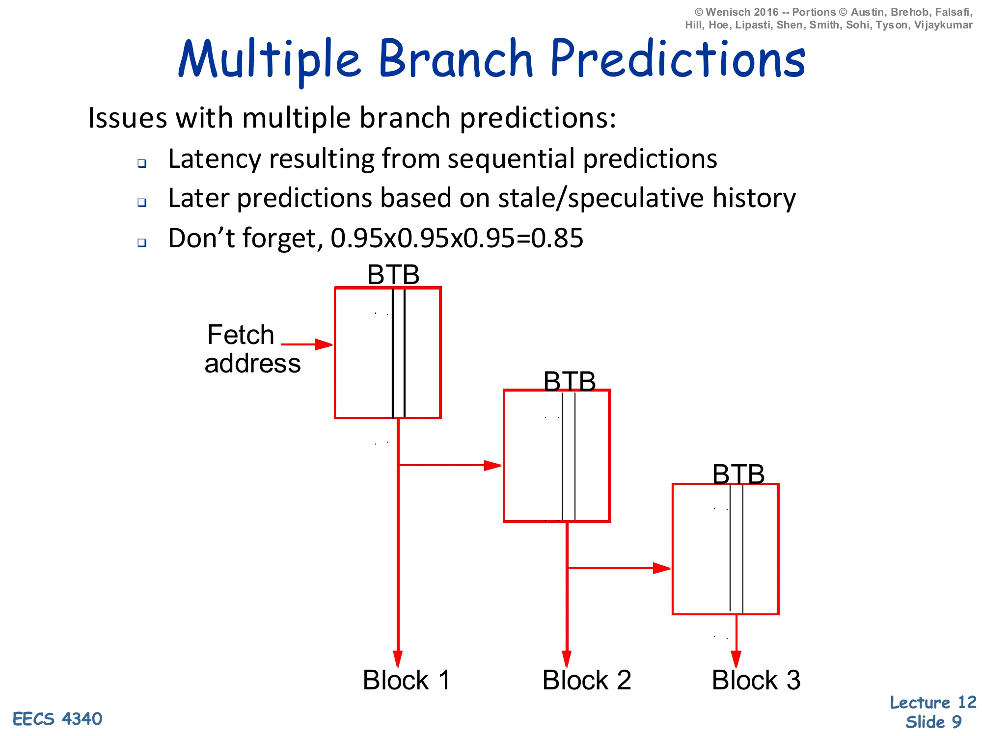
Multiple Branch Predictions

Issues with multiple branch predictions:

• Latency resulting from sequential predictions
• Later predictions based on stale/speculative history
• Don’t forget, $0.95 \times 0.95 \times 0.95 = 0.85$

Diagram: Fetch address feeds three cascaded BTB lookups producing Block 1, Block 2, Block 3.

Predicting several branches per cycle is harder than running one BTB/BHT lookup three times in series. First, the chained-lookup latency is the sum of three predictor delays; a multi-cycle predictor cannot keep up at all. Second, prediction $k+1$ depends on prediction $k$ — the global history fed into branch $k+1$ should reflect whatever direction was just predicted for branch $k$, but that bit is itself speculative, so each successive prediction is layered on more speculation and the predictor is operating on stale state by the time it makes prediction 3. Third, the slide’s arithmetic reminder cuts the most: per-branch accuracy compounds. Three 95%-accurate predictions yield only 85% confidence that the entire fetch window is correct, so a wider fetch with the same per-branch accuracy delivers progressively more wasted work per mispredict. Real implementations either widen the predictor table to issue several predictions in parallel from one indexed entry (slide 10), or sidestep the problem by storing already-traversed branch sequences in a trace cache (slide 11).

Examples of Multi-Branch Predictors

Slide 10

Show slide text

Examples of Multi-Branch Predictors

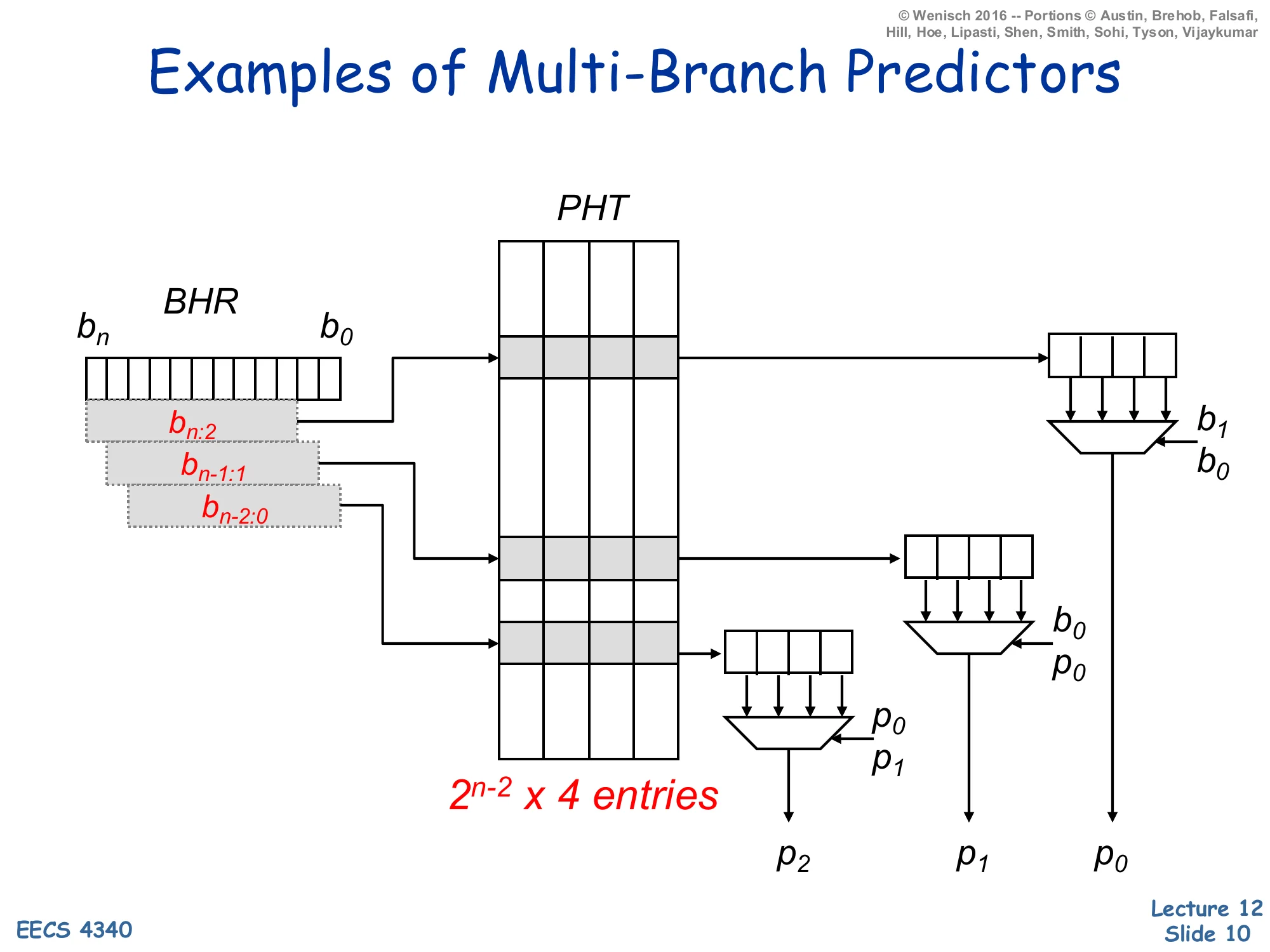
A single PHT of $2^{n-2} \times 4$ entries indexed by overlapping slices of the global BHR ($b_{n:2}$, $b_{n-1:1}$, $b_{n-2:0}$) produces three predictions $p_2, p_1, p_0$ in parallel. Each lookup yields a 4-wide row whose lanes are muxed by the next prediction(s):

• $p_0$ chosen by $b_1, b_0$
• $p_1$ chosen by $b_0, p_0$
• $p_2$ chosen by $p_0, p_1$

This diagram realizes a parallel multi-branch predictor by widening the pattern history table (PHT) so that one indexed row stores predictions for all $2^k$ possible directions of the next $k$ branches; only the first prediction is actually known when the lookup starts. Three slightly-shifted views of the global BHR each index a row of four 2-bit counters in parallel. The first prediction $p_0$ comes out immediately because the BHR slice $b_{n-2:0}$ together with $b_1, b_0$ identifies a fully-known counter. The second prediction $p_1$ uses the predicted outcome $p_0$ (fed forward through a mux) instead of waiting for the real branch to resolve; similarly $p_2$ uses both $p_0$ and $p_1$. The end result is three predictions per cycle at one PHT-access latency, at the cost of $4\times$ table width. The technique was popularized by Yeh, Marr, and Patt as the pattern-history-table multi-branch predictor; it is the architectural ancestor of the wider “ahead-pipelined” predictors used in modern wide-fetch cores. As before, gshare-style XOR-folding can be combined with this trick to cut PHT size.

Trace Cache Motivation

Slide 11

Show slide text

Trace Cache Motivation

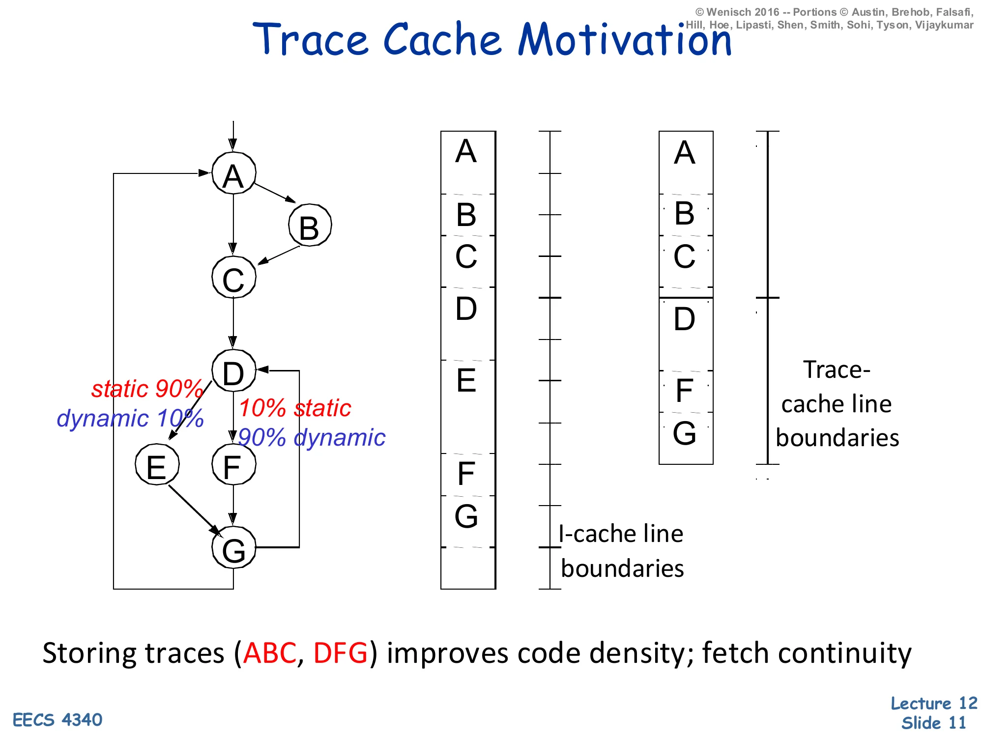
CFG nodes: A → B (static 90% / dynamic 10%) → C, then A → C; C → D; D → E (static 10% / dynamic 90%) or D → F → G; E → G; G → A.

• Traditional I-cache lays out blocks in static program order (A, B, C, D, E, F, G) split across I-cache line boundaries.
• Trace-cache packs the dynamic hot path (A, B, C, D, F, G) into a contiguous trace-cache line.

Storing traces (ABC, DFG) improves code density; fetch continuity.

A trace cache stores instructions in dynamic execution order rather than static program order. The control-flow graph on the slide has a hot dynamic path A→B→C→D→F→G even though the static layout interleaves the cold blocks E and the like. The middle column shows the I-cache view: blocks are laid out by virtual address so the hot path crosses several cache-line boundaries; on every taken branch the front end loses the rest of that line. The right column shows the trace-cache view: the runtime fetch sequence (A, B, C, then D, F, G) is captured as two contiguous trace-cache lines, each starting at a branch target. A single trace-cache lookup delivers a fetch-aligned run of instructions even though the original code straddled multiple basic blocks and predicted-taken branches. Pentium 4 famously stored decoded $\mu$ops in its trace cache; modern x86 cores still use a decoded-$\mu$op cache for the same reason. The cost is duplication: the same static block can appear in many traces, raising effective I-cache capacity pressure. The labels static 90% / dynamic 10% on the B and E edges remind you that profile-driven hot-path identification is what makes the trace cache worth the duplication.

Trace Cache Example

Slide 12

Show slide text

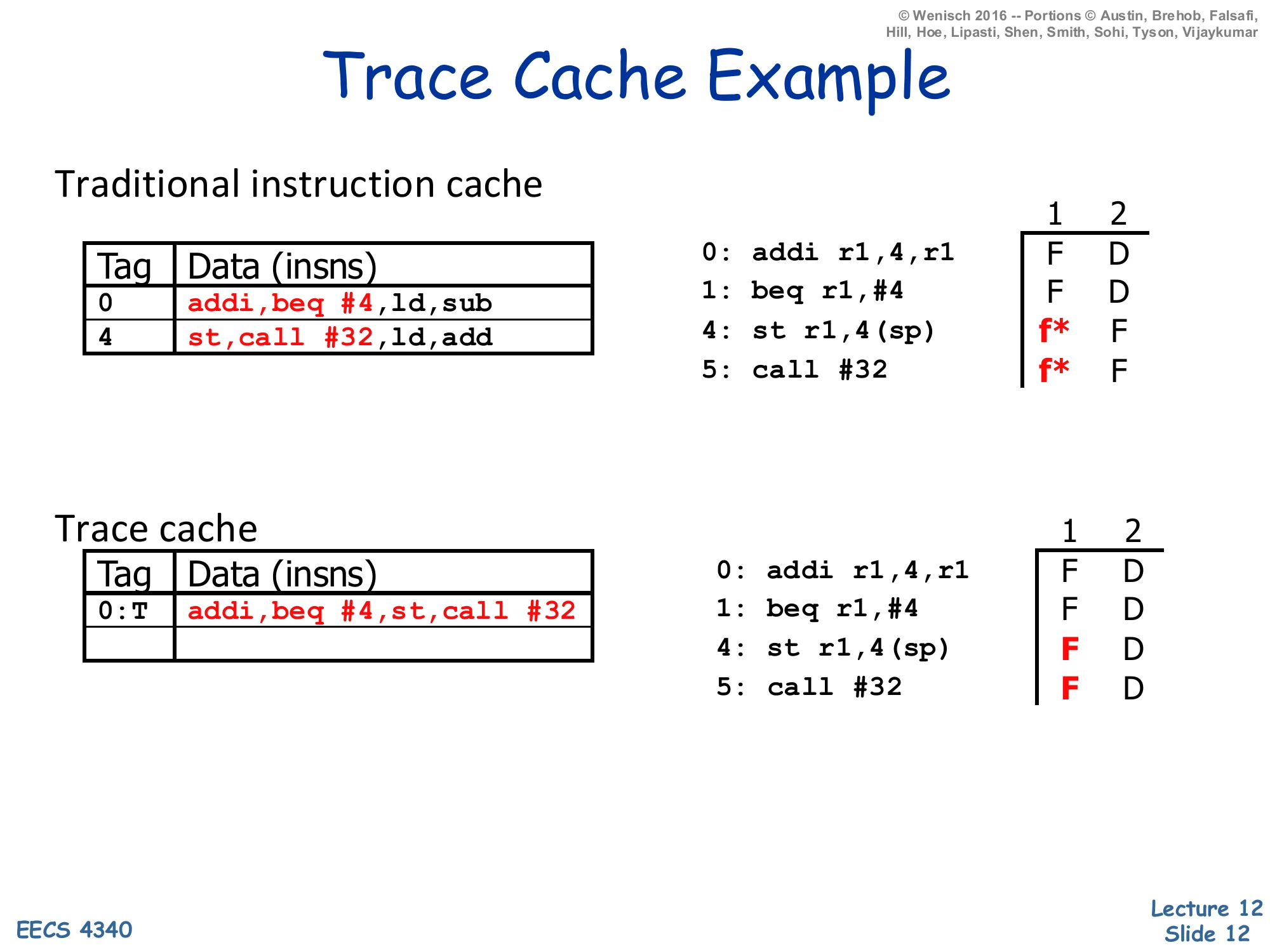
Trace Cache Example

Traditional instruction cache

Tag	Data (insns)
0	addi, beq #4, ld, sub
4	st, call #32, ld, add

Fetch trace for 0: addi r1,4,r1, 1: beq r1,#4, 4: st r1,4(sp), 5: call #32:

• Insn 0: F D
• Insn 1: F D
• Insn 4: f* (fetch bubble) F D
• Insn 5: f* F D

Trace cache

Tag	Data (insns)
0:T	addi, beq #4, st, call #32

Fetch trace:

• Insn 0: F D
• Insn 1: F D
• Insn 4: F D
• Insn 5: F D

This example makes the fetch-continuity benefit concrete. The traditional I-cache holds two static lines: line 0 is {addi, beq #4, ld, sub} and line 4 is {st, call #32, ld, add}. When beq at PC 1 is predicted taken to PC 4, the two predicted-taken instructions (ld and sub after beq) are dead and st, call #32 start in the next fetch slot — the timing column shows two f* bubbles where fetch must wait a cycle for the new line and then squash the dead instructions. The trace cache uses a tag of 0:T (PC 0 with the branch predicted taken), and its line packs the four instructions actually executed in dynamic order: addi, beq #4, st, call #32. Now all four hit in one cycle and decode in the next — the fetch bubbles vanish. Notice that the trace-cache tag includes the prediction direction, so a different prediction at PC 0 would miss this line and trigger a different trace lookup; this is how the trace cache expresses path-sensitivity at the cost of duplicating the cold-path version of the same addi/beq pair.

Memory Systems: Basic Caches

Slide 13

Memory Systems

Slide 14

Show slide text

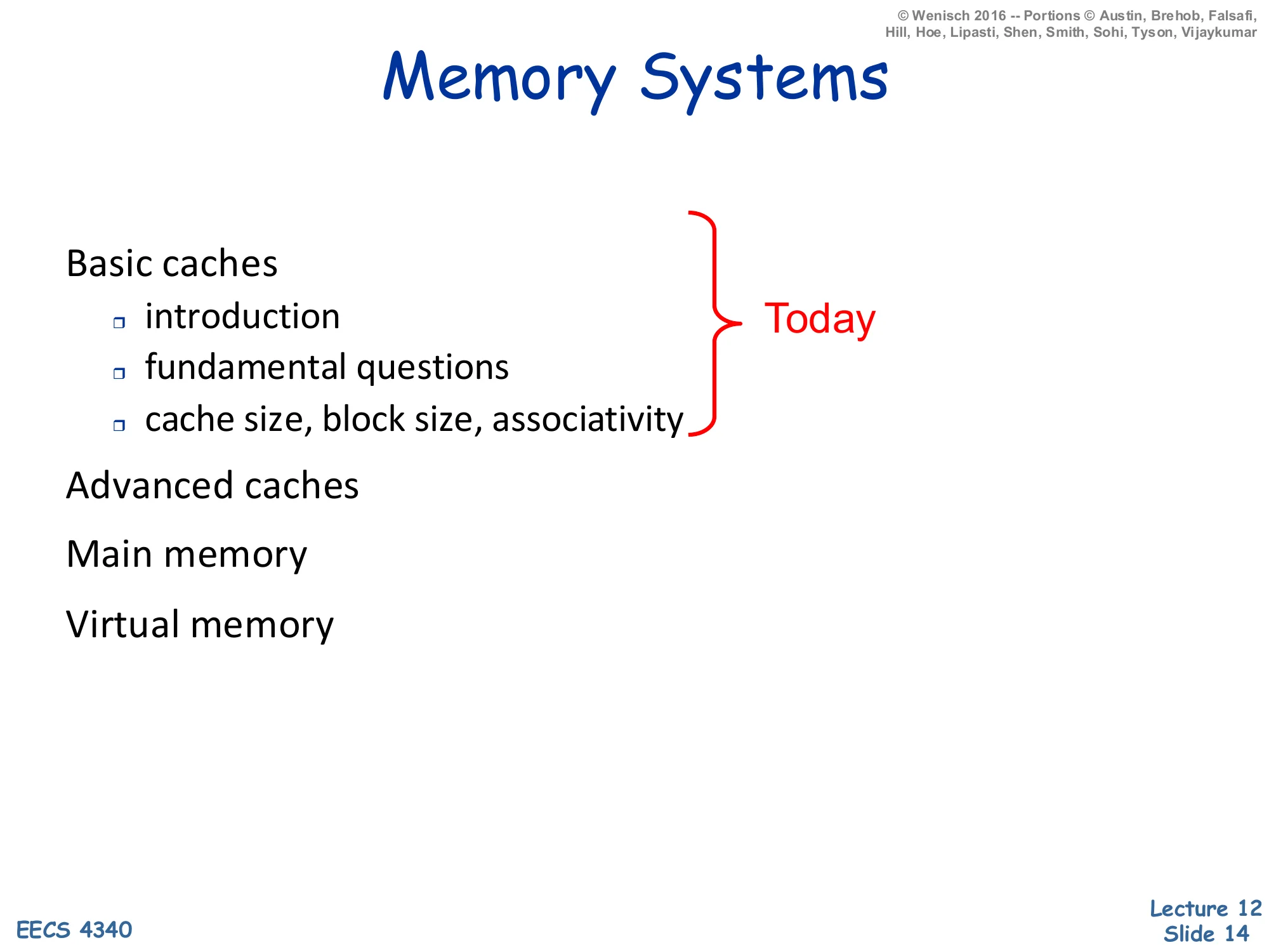
Memory Systems

Basic caches (Today)

• introduction
• fundamental questions
• cache size, block size, associativity

Advanced caches

Main memory

Virtual memory

This is the roadmap for the memory-systems sub-unit. Today’s lecture covers basic caches: why caches exist (the processor-memory gap on the next slide), the four fundamental design questions (placement, replacement, write strategy, bookkeeping) introduced abstractly, and the three knobs that govern miss rate — cache size $C$, block size $b$, and associativity $a$. Later memory lectures will cover advanced caches (multi-level hierarchies, victim caches, prefetching, non-blocking caches), main memory (DRAM organization and timing), and virtual memory (TLBs, page tables, and address translation). Keeping this scaffold in mind helps when individual slides reference “the next lecture” — most of the optimizations only make sense once you have the basic-cache vocabulary nailed down.

Motivation

Slide 15

Show slide text

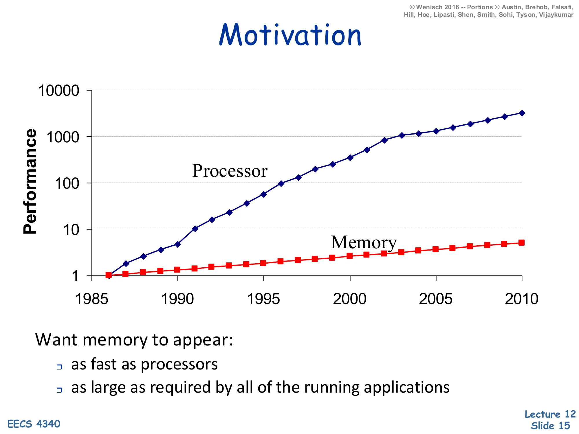
Motivation

Log-scale performance plot 1985–2010: processor performance grows from 1 to ~3000×, while memory performance grows from 1 to ~5×.

Want memory to appear:

• as fast as processors
• as large as required by all of the running applications

The classic processor–memory gap chart explains why caches exist. Between 1985 and 2010, single-thread CPU performance improved by roughly $3000\times$ (driven by frequency scaling and microarchitectural ILP), while DRAM access time improved by only ~$5\times$. On a log scale the two curves diverge dramatically, and the multiplicative gap by 2010 is on the order of $600\times$. A program that issues a load every few instructions and waits hundreds of cycles for DRAM cannot benefit from any frequency or IPC gains; the processor would simply stall. The two design goals at the bottom — as fast as the processor and as large as the applications need — are mutually exclusive at any single technology point: SRAM is fast but expensive per bit, DRAM is large but slow, and disk is huge but glacial. The memory hierarchy resolves the contradiction by stacking these technologies and exploiting locality so the common case hits the small-and-fast layer.

Memory Hierarchy

Slide 16

Show slide text

Memory Hierarchy

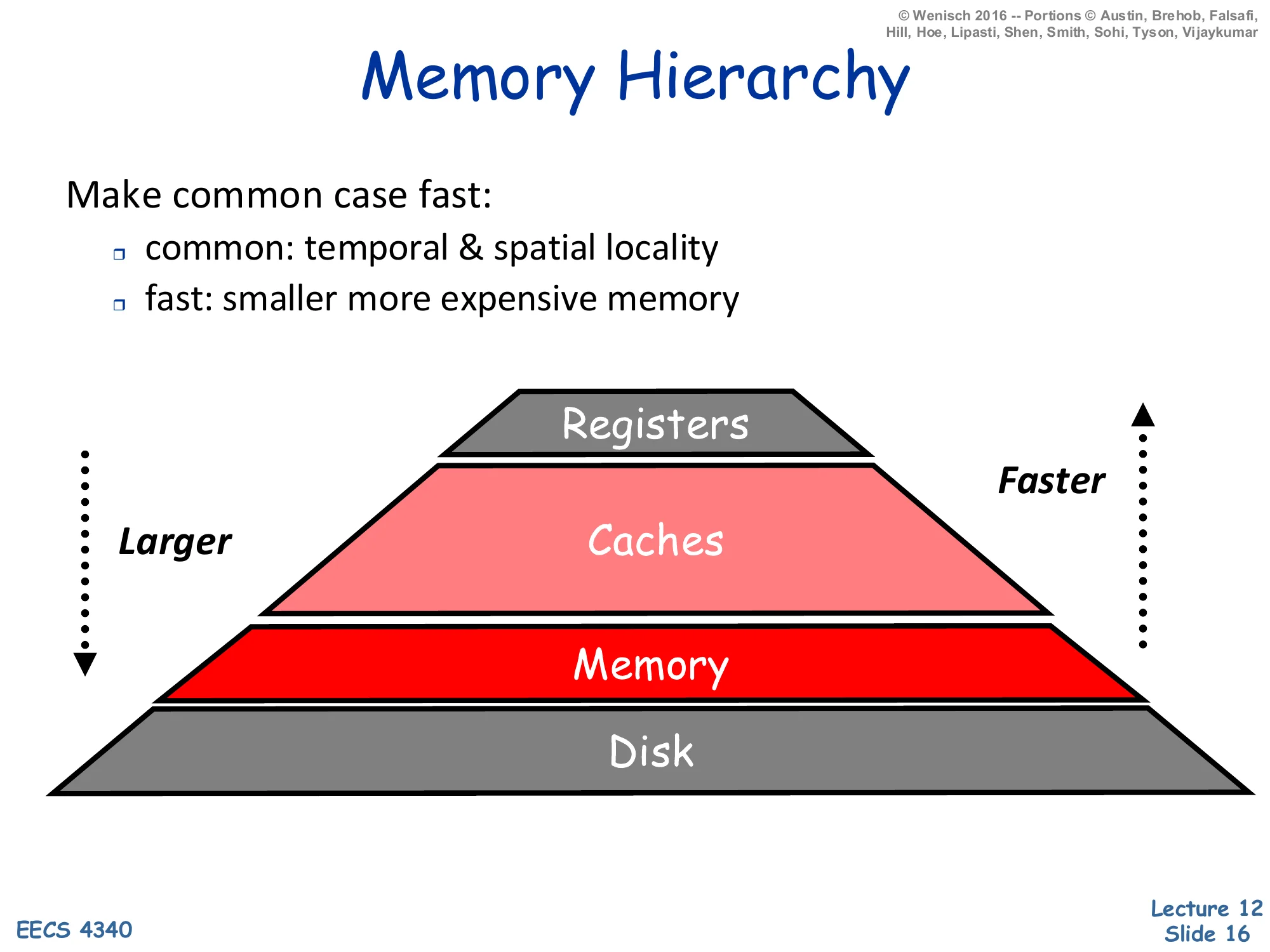
Make common case fast:

• common: temporal & spatial locality
• fast: smaller more expensive memory

Pyramid: Registers (smallest, fastest) → Caches → Memory → Disk (largest, slowest). Larger going down, faster going up.

The memory hierarchy applies the make-the-common-case-fast principle to addresses. Programs exhibit two flavors of locality. Temporal locality says that if address $A$ was just accessed it will likely be accessed again soon (loop induction variables, hot stack frames). Spatial locality says that if $A$ was just accessed, addresses near $A$ will also be accessed soon (sequential array sweeps, instruction streams). The pyramid stacks technologies by speed/cost: registers (~1 cycle, hundreds of bytes) sit at the top, then on-chip caches (~1–30 cycles, kilobytes to megabytes), then DRAM main memory (~100–300 cycles, gigabytes), then disk (millions of cycles, terabytes). Each layer caches data from the layer below it; a hit at level $i$ avoids paying the latency of level $i+1$. Provided locality is high — i.e. the working set of recently used addresses fits in some intermediate level — average access time is dominated by the fastest level, even though the absolute capacity is set by the slowest. Registers are an ISA-visible feature managed by the compiler; everything below is automatically managed by hardware (caches) or the OS+hardware (virtual memory).

Storage Hierarchies

Slide 17

Show slide text

Storage Hierarchies

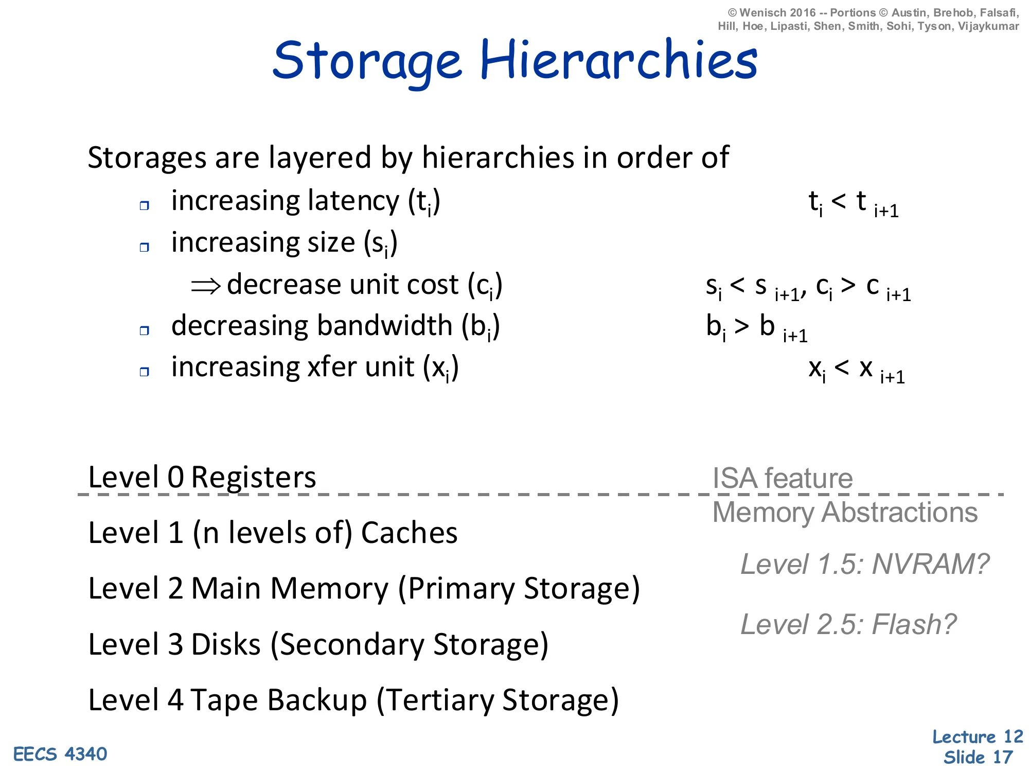
Storages are layered by hierarchies in order of:

• increasing latency $(t_i)$: $t_i < t_{i+1}$
• increasing size $(s_i)$ $\Rightarrow$ decrease unit cost $(c_i)$: $s_i < s_{i+1}$, $c_i > c_{i+1}$
• decreasing bandwidth $(b_i)$: $b_i > b_{i+1}$
• increasing xfer unit $(x_i)$: $x_i < x_{i+1}$

Levels:

• Level 0: Registers (ISA feature)
• Level 1: ($n$ levels of) Caches
• Level 2: Main Memory (Primary Storage)
• Level 3: Disks (Secondary Storage)
• Level 4: Tape Backup (Tertiary Storage)

Memory abstractions: Level 1.5: NVRAM? Level 2.5: Flash?

This slide formalizes the hierarchy with four monotonicity properties: as you descend, latency $t_i$ goes up, capacity $s_i$ goes up, unit cost $c_i$ goes down, bandwidth $b_i$ goes down (because the wider, slower technologies feed fewer requests per second), and the transfer unit $x_i$ — the granularity of data movement — goes up. That last property is the architectural justification for cache blocks: when you spend ~100 cycles to access DRAM, you may as well bring back 64 contiguous bytes (a typical $x_2$) instead of one word, because amortizing the per-access overhead lets the bandwidth-limited link do useful work. The named levels show the canonical 5-tier hierarchy. Registers are the only level explicitly visible to the ISA — every read or write is encoded in the instruction. Levels 1–4 are memory abstractions invisible to software: caches are managed by hardware; main memory and disk are managed by the OS via virtual memory. The italicized level 1.5 (NVRAM) and 2.5 (Flash/SSD) are recent technologies that don’t fit cleanly into the 5-tier picture but slot between SRAM/DRAM and DRAM/HDD respectively.

Processor/Memory Boundaries

Slide 18

Show slide text

Processor/Memory Boundaries

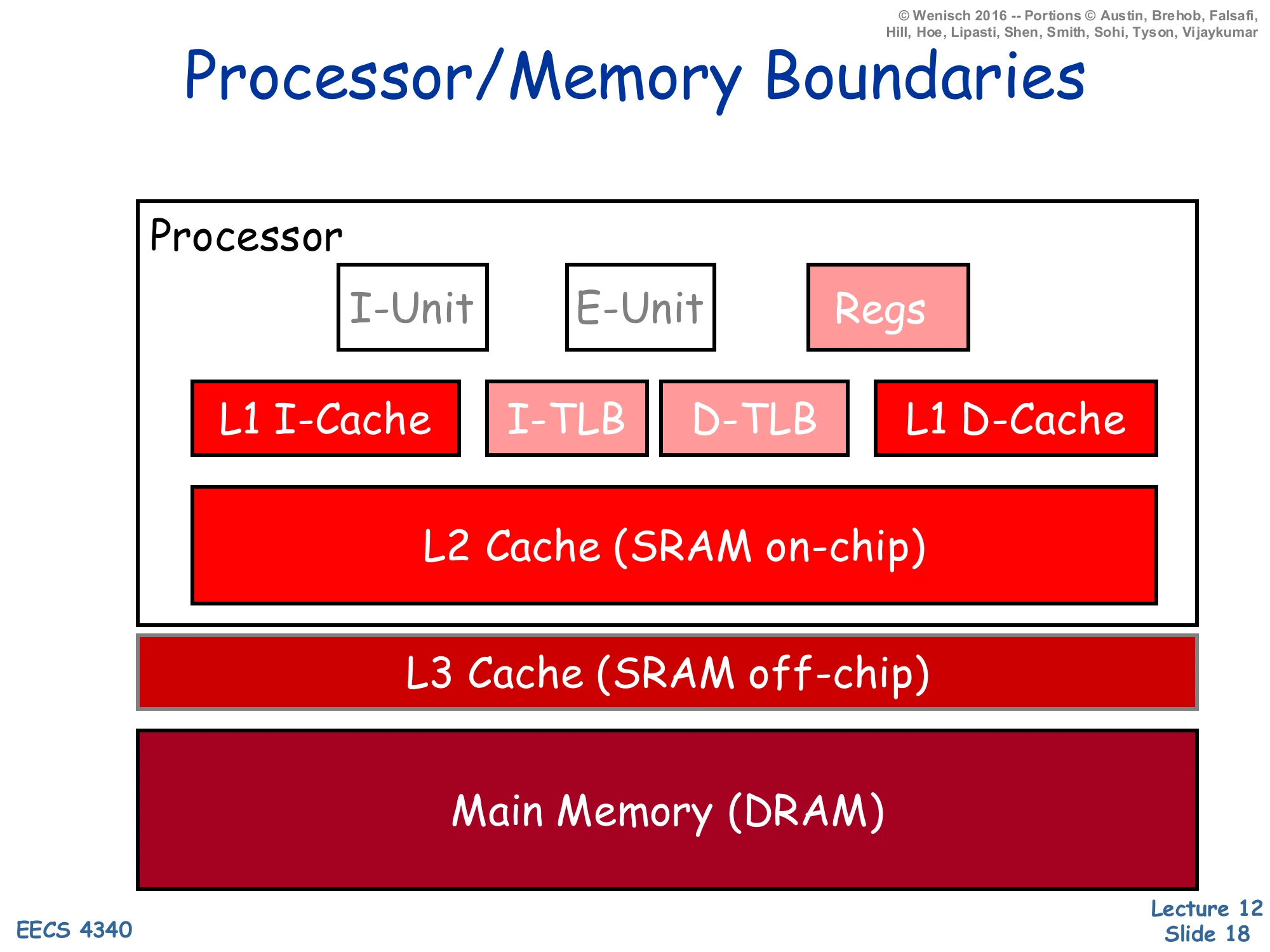
On-chip processor:

• I-Unit, E-Unit, Regs
• L1 I-Cache, I-TLB, D-TLB, L1 D-Cache
• L2 Cache (SRAM on-chip)

Off-chip:

• L3 Cache (SRAM off-chip)
• Main Memory (DRAM)

This block diagram identifies the physical boundaries that map onto the storage hierarchy. The processor die holds: the I-Unit (instruction fetch/decode/branch), the E-Unit (execute/ALU), the architectural register file, split L1 instruction and data caches (Harvard organization, see slide 39), the I-TLB and D-TLB for address translation, and a unified on-chip L2 cache. In modern designs the L3 is usually also on-chip (the slide reflects an older tier where L3 was off-chip SRAM); main memory is always off-chip DRAM. Latency rises sharply at every boundary: ~1 cycle for registers, 3–5 cycles for L1, 10–15 cycles for L2, 30–50 cycles for L3, and 200+ cycles for DRAM. Crossing the chip boundary alone costs tens of cycles because of pad drivers, off-chip wire delay, and the bus protocol. The TLB sits next to the L1s because virtual addresses must be translated before the cache index can be computed (or in parallel for VIPT caches); we’ll cover that in the virtual-memory lecture.

Caches

Slide 19

Show slide text

Caches

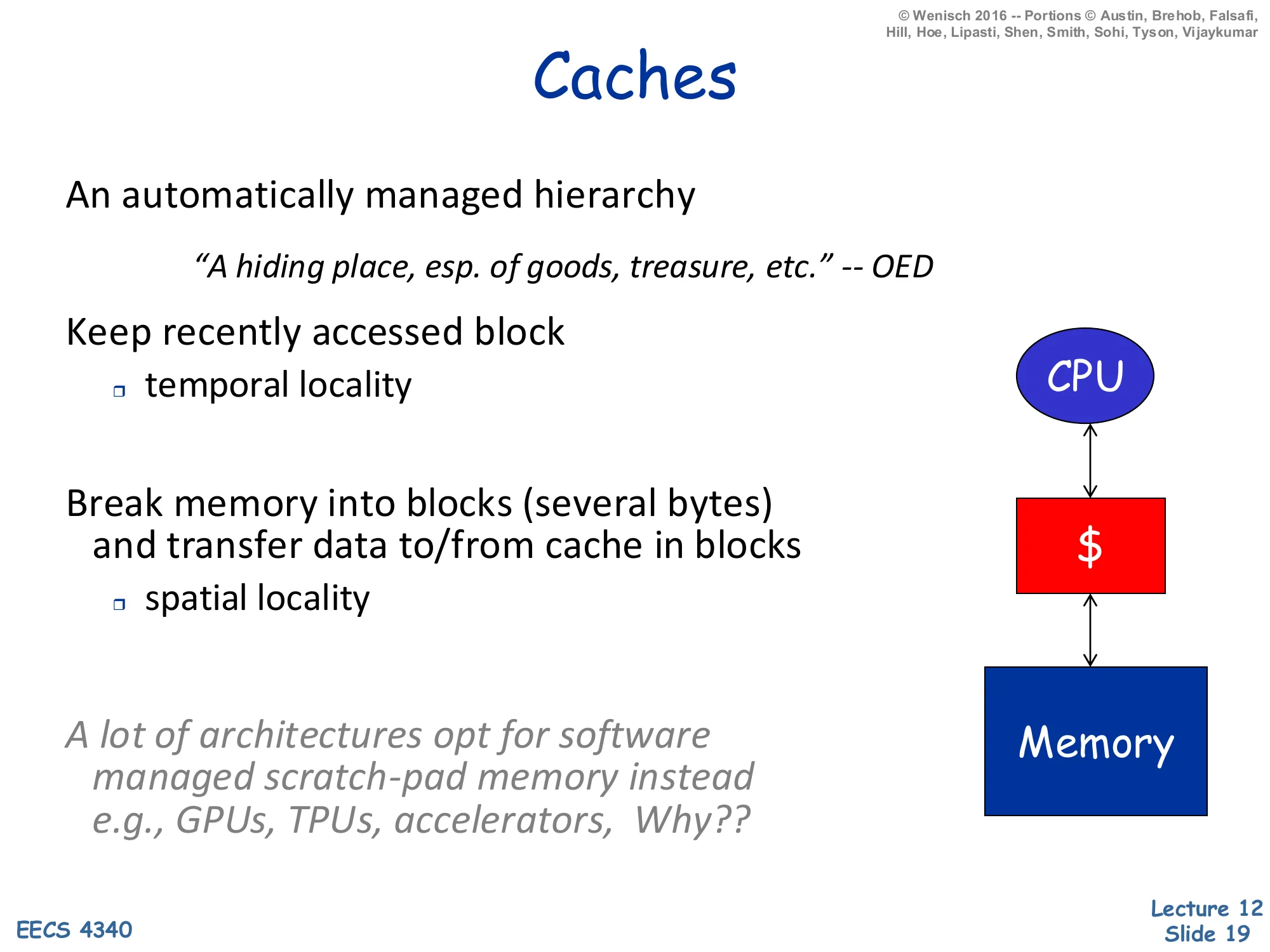
An automatically managed hierarchy

“A hiding place, esp. of goods, treasure, etc.” — OED

Keep recently accessed block

• temporal locality

Break memory into blocks (several bytes) and transfer data to/from cache in blocks

• spatial locality

A lot of architectures opt for software managed scratch-pad memory instead, e.g., GPUs, TPUs, accelerators. Why??

A cache is automatic — neither the compiler nor the programmer decides what stays — and it exploits both flavors of locality. Temporal locality is exploited by the hit/replace policy: a block that was just accessed stays resident until evicted, so the same block can be re-read for free. Spatial locality is exploited by transferring data in blocks (typically 32–128 bytes) rather than single bytes; once you pay the access penalty of going to the next level, you might as well bring back neighbors. The italicized aside about scratch-pad memories on GPUs/TPUs is a thought exercise: accelerators have well-understood, statically tile-able access patterns (matrix-matrix multiply, convolutional kernels), so a software-managed on-chip SRAM eliminates the tag/replacement overhead and gives the programmer deterministic latency. CPUs cannot make those assumptions about general-purpose code, so they pay the area and energy cost of automatic caches in exchange for transparency.

Cache (Abstractly)

Slide 20

Show slide text

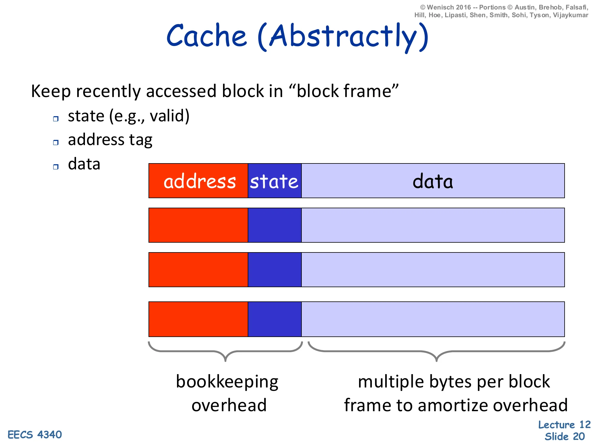
Cache (Abstractly)

Keep recently accessed block in “block frame”

• state (e.g., valid)
• address tag
• data

Layout per frame: address | state | data

• Bookkeeping overhead: address tag + state
• Multiple bytes per block frame to amortize overhead

A cache entry — called a block frame — has three fields: the address tag identifying which memory block currently lives there, state bits (at minimum a valid bit, plus a dirty bit for write-back caches and coherence state for shared caches), and the data itself. The tag and state together are the bookkeeping overhead, and a key engineering decision is to amortize that overhead by making the data field much wider than a single word: a 64-byte data field with a ~25-bit tag and a few state bits has only $\sim 4\%$ overhead, while a 4-byte data field with the same tag has $\sim 50\%$ overhead. This is the structural reason caches use multi-byte blocks instead of word-sized entries — and it’s the same reason that pushed up cache-line sizes from 16 bytes in the 80s to 64–128 bytes today as tags and ECC overhead grew.

Cache (Abstractly) — Lookup Algorithm

Slide 21

Show slide text

Cache (Abstractly) — Lookup

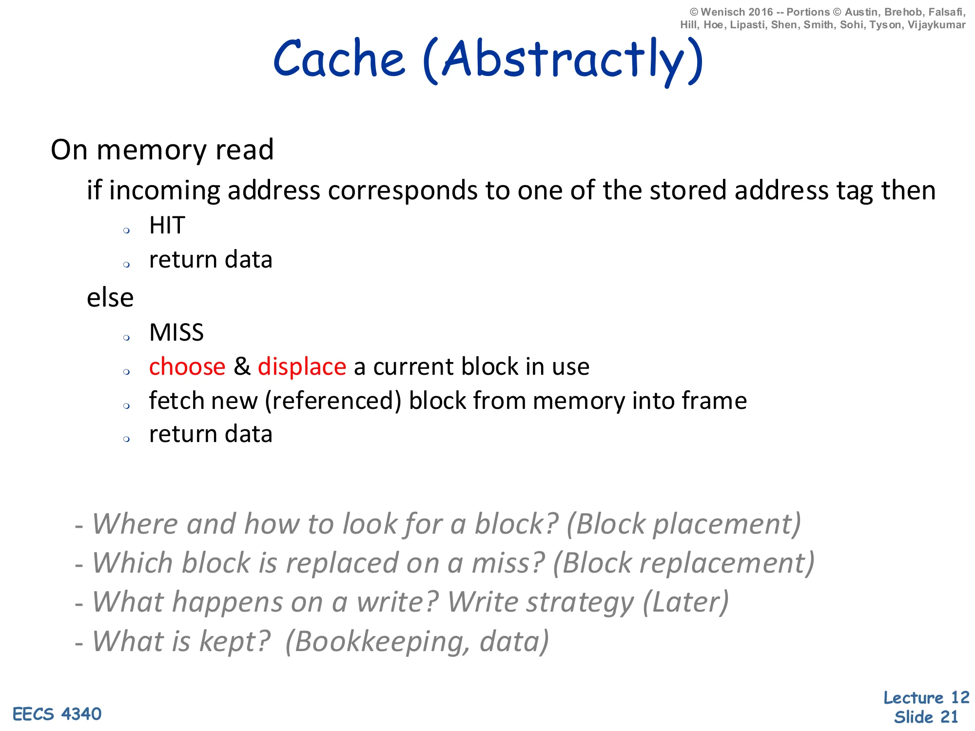
On memory read

• if incoming address corresponds to one of the stored address tags then
  • HIT
  • return data
• else
  • MISS
  • choose & displace a current block in use
  • fetch new (referenced) block from memory into frame
  • return data

Four fundamental questions:

• Where and how to look for a block? (Block placement)
• Which block is replaced on a miss? (Block replacement)
• What happens on a write? Write strategy (Later)
• What is kept? (Bookkeeping, data)

The hit path is trivial: compare the incoming address tag to stored tags, return data on match. The miss path triggers four design decisions, listed at the bottom, that organize the rest of the lecture. Block placement asks which set/frame an incoming block can occupy — direct-mapped, set-associative, or fully associative (slide 27). Block replacement asks which existing block to evict when a new block displaces it (LRU, NMRU, random — slide 34). Write strategy asks what happens on writes: write-through vs write-back, and write-allocate vs no-write-allocate (slides 35–36). Bookkeeping asks what state bits accompany each block (valid, dirty, replacement-policy bits, coherence state). The reading sequence — placement, replacement, writes — is the standard organization in Hennessy & Patterson, and most cache-design problem sets follow exactly these four questions.

Terminology

Slide 22

Show slide text

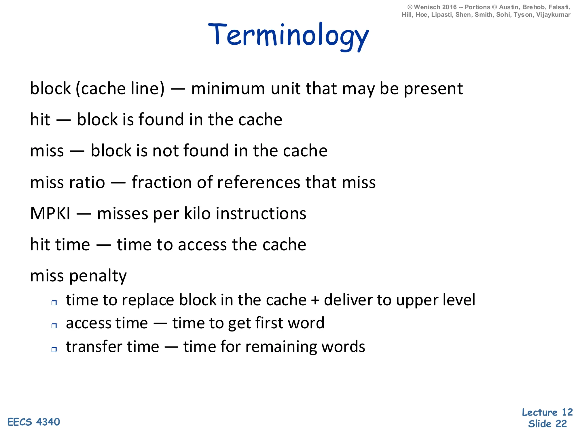
Terminology

• block (cache line) — minimum unit that may be present
• hit — block is found in the cache
• miss — block is not found in the cache
• miss ratio — fraction of references that miss
• MPKI — misses per kilo instructions
• hit time — time to access the cache
• miss penalty
  • time to replace block in the cache + deliver to upper level
  • access time — time to get first word
  • transfer time — time for remaining words

These are the words that appear in every cache problem. A block (cache line) is the minimum quantum the cache can store and transfer; you cannot have half a block resident. A hit finds the block, a miss does not. Miss ratio (a fraction in $[0,1]$) is the standard performance metric for cache designs whose hit time is fixed; MPKI (misses per thousand instructions) is preferred for architectural comparisons because it normalizes by program work rather than by reference count, and it’s the natural denominator for cycles-lost-to-memory budgeting. Hit time is the latency to return data on a hit. Miss penalty breaks down further into access time (latency until the first word arrives) and transfer time (the remaining words of the block); high-bandwidth memory channels make transfer time small relative to access time, so block size is often chosen so the entire block fits in one access burst. The next slide combines hit time and miss penalty into average access time, the key analytic model.

Cache Performance

Slide 23

Show slide text

Cache Performance

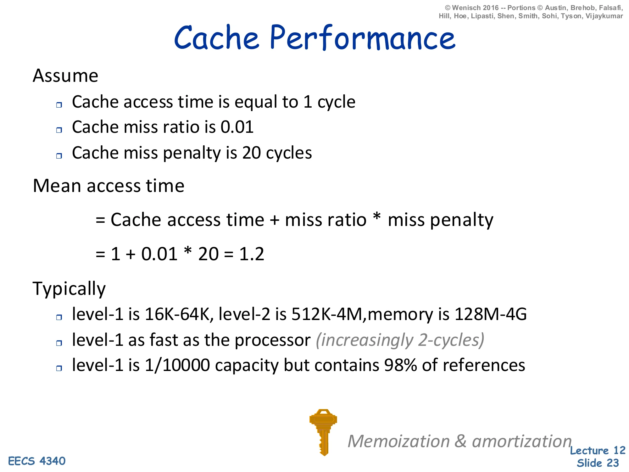
Assume

• Cache access time is equal to 1 cycle
• Cache miss ratio is 0.01
• Cache miss penalty is 20 cycles

Mean access time

$\text{AMAT} = \text{Cache access time} + \text{miss ratio} \times \text{miss penalty}$

$\text{AMAT} = 1 + 0.01 \times 20 = 1.2$

Typically

• level-1 is 16K–64K, level-2 is 512K–4M, memory is 128M–4G
• level-1 as fast as the processor (increasingly 2-cycles)
• level-1 is 1/10000 capacity but contains 98% of references

Memoization & amortization

AMAT (average memory access time) is the cache designer’s iron law. The base form is hit_time + miss_rate × miss_penalty; with the slide’s numbers, a 1-cycle hit time and 1% miss rate against a 20-cycle DRAM yields 1.2 cycles per reference — only 20% slower than a perfect cache despite a 20× speed gap. This is the magic of locality: the L1 holds $\frac{1}{10{,}000}$ of memory but absorbs 98% of references, so the slow level rarely matters. AMAT generalizes recursively: for a multi-level hierarchy, replace the leaf miss penalty with the AMAT of the next level. For two levels, $\text{AMAT} = t_{L1} + m_{L1}(t_{L2} + m_{L2}\,t_{mem})$. Note that the L1 miss rate alone does not capture system performance — the local miss rate (misses at L1 ÷ accesses to L1) and the global miss rate (misses at L2 ÷ accesses to L1) describe different things, and many textbook problems exploit the distinction. The footnote memoization & amortization names the underlying ideas: caching is just dynamic memoization, and the multi-byte block amortizes the per-miss overhead across spatial neighbors.

Fundamental Cache Parameters that Affect Miss Rate

Slide 24

Show slide text

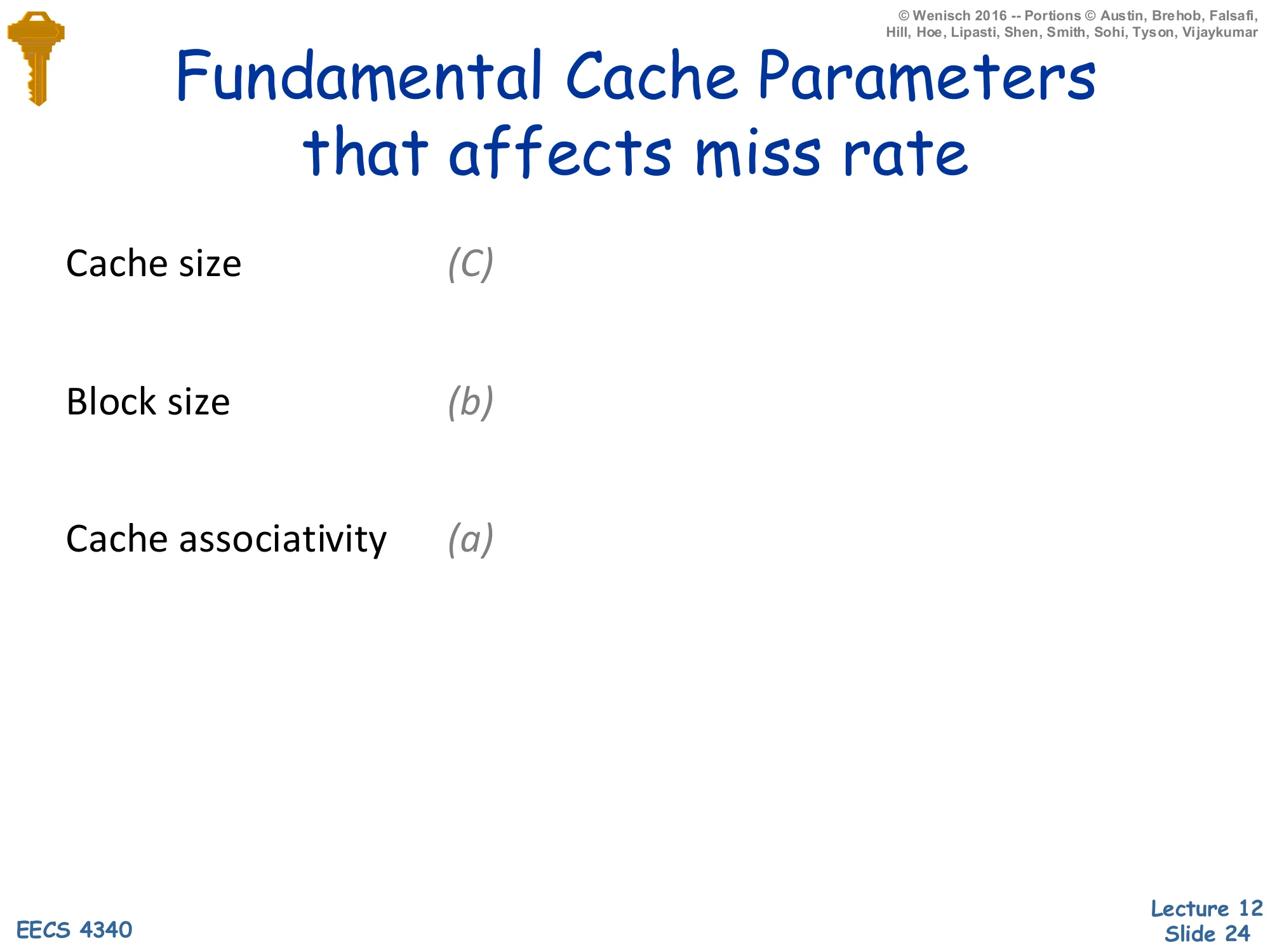
Fundamental Cache Parameters that Affect Miss Rate

• Cache size $(C)$
• Block size $(b)$
• Cache associativity $(a)$

Three parameters together determine miss rate at any given workload: total cache capacity $C$, block size $b$, and associativity $a$. They interact: $C = a \times b \times \#\text{sets}$, so changing one while “holding the others constant” usually means changing the number of sets. The next three slides explore each parameter in isolation while holding the other two fixed. The reason these three matter (and not, say, replacement policy) is that they each map onto a different one of the 3 Cs miss taxonomy: capacity misses (fixed by larger $C$), compulsory misses (reduced by larger $b$ via spatial prefetching of cold-block neighbors), and conflict misses (reduced by larger $a$). The 3 Cs framework is not on this slide but is the standard pedagogical scaffold; H&P will cover it in the advanced-caches lecture.

Cache Size

Slide 25

Show slide text

Cache Size

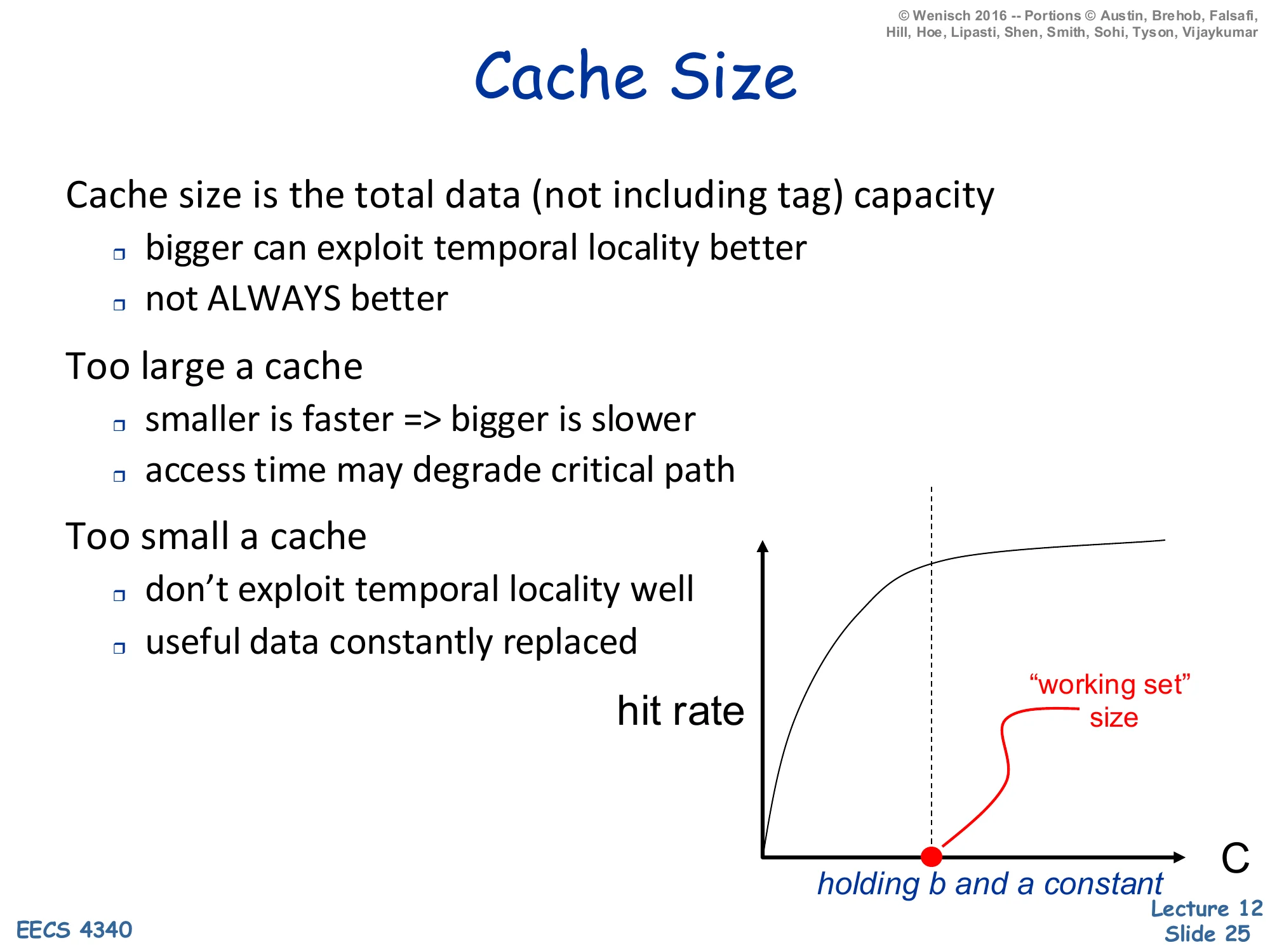
Cache size is the total data (not including tag) capacity

• bigger can exploit temporal locality better
• not ALWAYS better

Too large a cache

• smaller is faster $\Rightarrow$ bigger is slower
• access time may degrade critical path

Too small a cache

• don’t exploit temporal locality well
• useful data constantly replaced

Hit-rate vs. $C$ curve: concave, knee at “working set” size, holding $b$ and $a$ constant.

Larger caches reduce miss rate, but with diminishing returns and a real downside on hit time. The hit-rate curve is concave: doubling capacity from 1KB to 2KB might add ten percentage points; doubling from 1MB to 2MB might add one. The knee of the curve corresponds to the working set — once the cache holds the application’s hot footprint, further capacity buys little. The downside is that bigger SRAM has longer wire delays and decoder fan-out, so access time grows roughly with $\sqrt{C}$. Above some critical $C$ the L1 hit time would exceed the rest of the pipeline’s clock budget and force the CPU to slow down. This is why modern designs split capacity across multiple levels — small fast L1, larger slower L2, very large L3 — rather than trying to make one giant L1. The slide’s holding $b$ and $a$ constant annotation is important: in practice you often increase $C$ by adding sets while keeping block size and associativity fixed, which preserves the per-set tag-comparison cost.

Block Size

Slide 26

Show slide text

Block Size

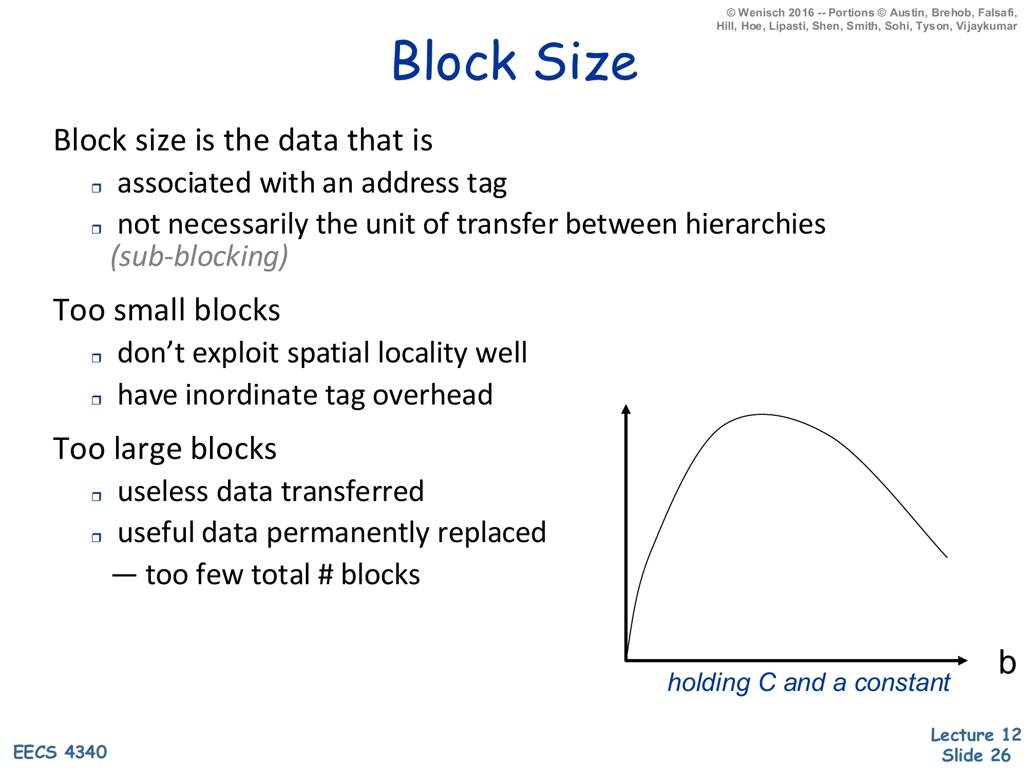
Block size is the data that is

• associated with an address tag
• not necessarily the unit of transfer between hierarchies (sub-blocking)

Too small blocks

• don’t exploit spatial locality well
• have inordinate tag overhead

Too large blocks

• useless data transferred
• useful data permanently replaced
  • too few total # blocks

Hit-rate vs. $b$ curve: unimodal — rises with $b$ then falls, holding $C$ and $a$ constant.

Block size is the spatial-locality dial. Tiny blocks (one word per tag) waste tag/state area and gain nothing from prefetching neighbors; the curve rises sharply as $b$ increases up to the working set’s effective spatial-locality footprint. Past that knee the curve falls again, because given fixed cache capacity $C$ a larger block size means $C/b$ fewer blocks total — the cache holds proportionally fewer distinct addresses, so capacity and conflict misses both rise. The two failure modes are useless data transferred (you brought back 128 bytes but only used 8) and useful data evicted (the larger block kicked out two valuable smaller blocks). The optimal $b$ depends on the workload’s spatial-locality profile and is empirically 32–128 bytes for most general-purpose code. The italicized sub-blocking note is a refinement: you can keep a large block for tag-amortization purposes but transfer only the sub-block actually requested, which makes the unit-of-transfer smaller than the unit-of-tag and lets you have your cake and eat it on the bandwidth side.

Associativity

Slide 27

Show slide text

Associativity

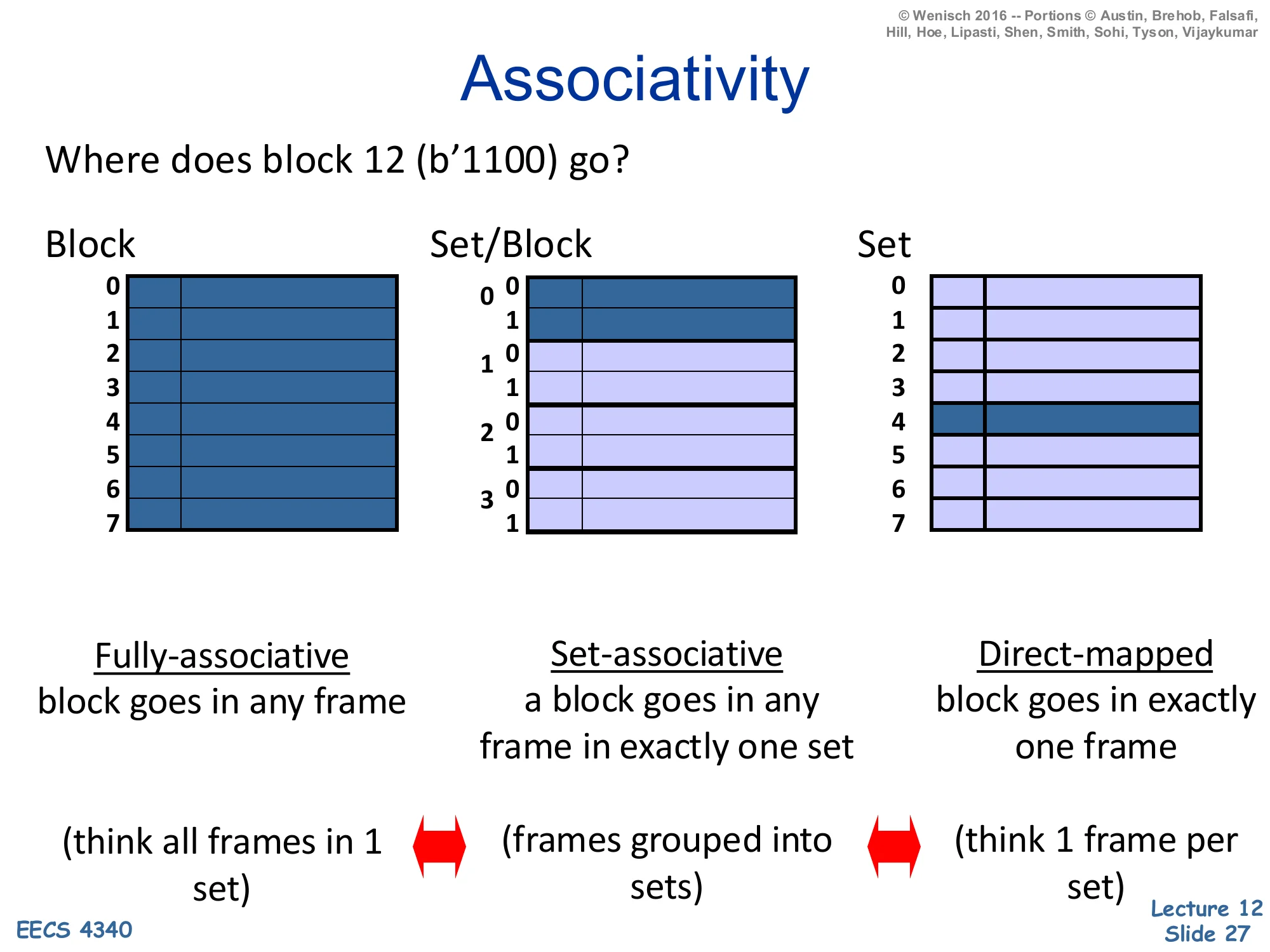
Where does block 12 (b’1100) go?

• Fully-associative — block goes in any frame (think all frames in 1 set)
• Set-associative — a block goes in any frame in exactly one set (frames grouped into sets)
• Direct-mapped — block goes in exactly one frame (think 1 frame per set)

Associativity tells the cache where a block may live. The slide visualizes the same eight frames under three organizations using block 12 = $1100_2$. Fully associative: one giant set, block 12 may occupy any of the eight frames; the lookup must compare the tag against all eight in parallel. Set-associative (here 2-way × 4 sets): block 12’s index = $12 \bmod 4 = 0$ selects set 0, and within set 0 the block may live in either of two frames. Direct-mapped: 8 sets of 1 frame each, block 12’s index = $12 \bmod 8 = 4$ pins it to frame 4 with no choice. Direct-mapped is fastest (one tag compare, no mux) but vulnerable to conflict misses when two hot addresses map to the same frame. Fully associative has zero conflict misses but $N$-way tag compare hardware grows linearly with $N$ and is impractical past a few hundred entries (which is why TLBs and victim caches use full associativity, while data caches use 4–16-way). The two double-headed arrows in the slide remind you that direct-mapped and fully-associative are the two extremes of set-associative.

Impact of Associativity

Slide 28

Show slide text

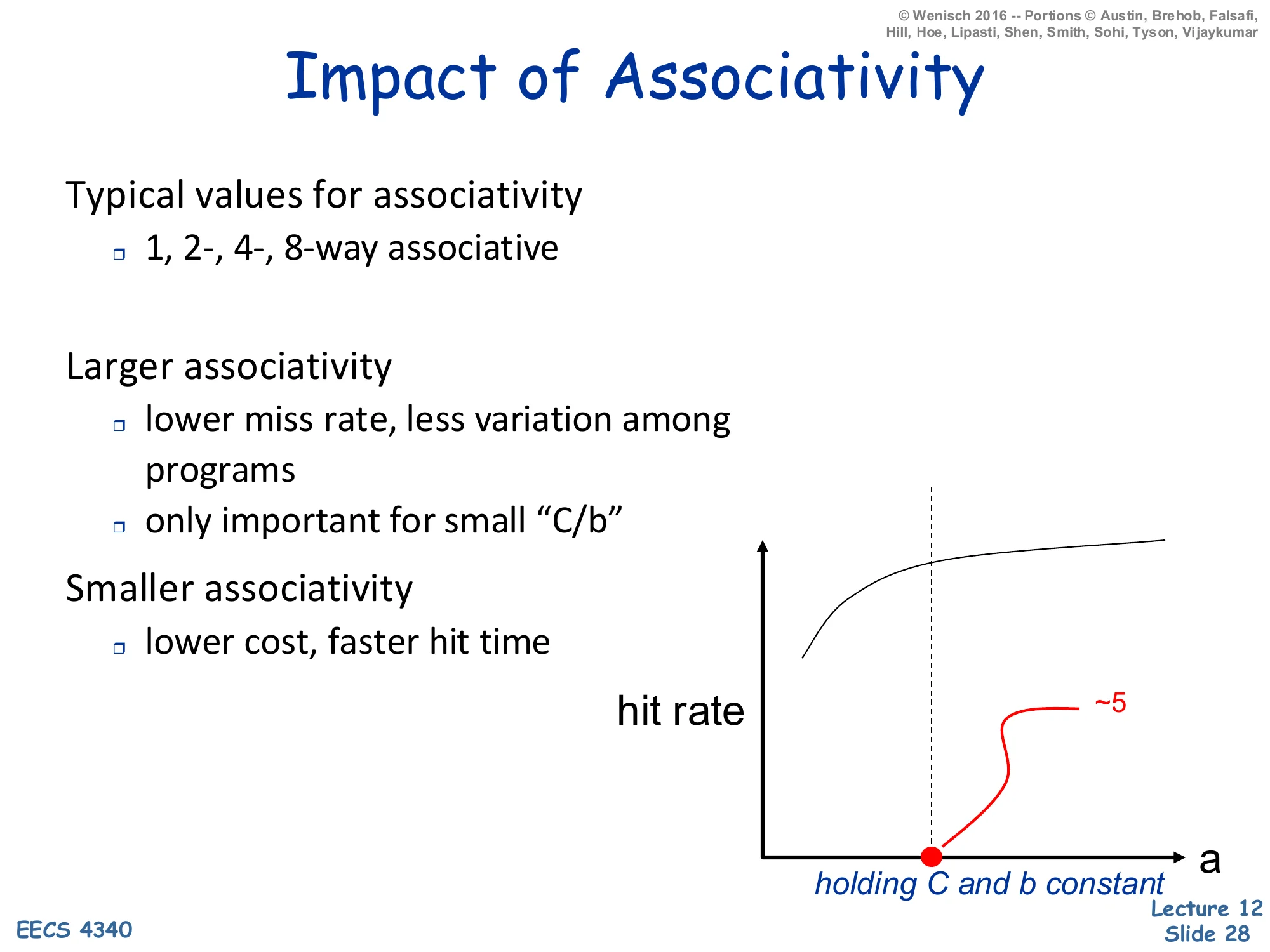
Impact of Associativity

Typical values for associativity

• 1, 2-, 4-, 8-way associative

Larger associativity

• lower miss rate, less variation among programs
• only important for small "$C/b$"

Smaller associativity

• lower cost, faster hit time

Hit-rate vs. $a$ curve: concave, knee at $a \approx 5$, holding $C$ and $b$ constant.

Associativity is the conflict-miss dial, but its returns saturate fast. Going from direct-mapped (1-way) to 2-way typically eliminates the bulk of conflict misses; 2-way to 4-way adds a smaller benefit; beyond about 4–8 ways the curve is essentially flat — the slide’s annotation $\sim 5$ at the knee captures this. The only important for small $C/b$ note is the deeper truth: when the cache has many sets (large $C/b$), random hashing of addresses to sets is already nearly uniform and conflicts are rare; associativity matters most for caches with few sets, like a small L1 with a large block size. Hit-time and area cost grow with $a$ (more parallel tag comparators, wider mux), so the design sweet spot is the smallest associativity that absorbs the workload’s conflicts. Hence the typical range — 1-way (direct-mapped, common in the 90s and still used in some embedded designs), 2- or 4-way (most modern L1s), 8- or 16-way (L2/L3).

Direct Mapped Caches

Slide 29

Show slide text

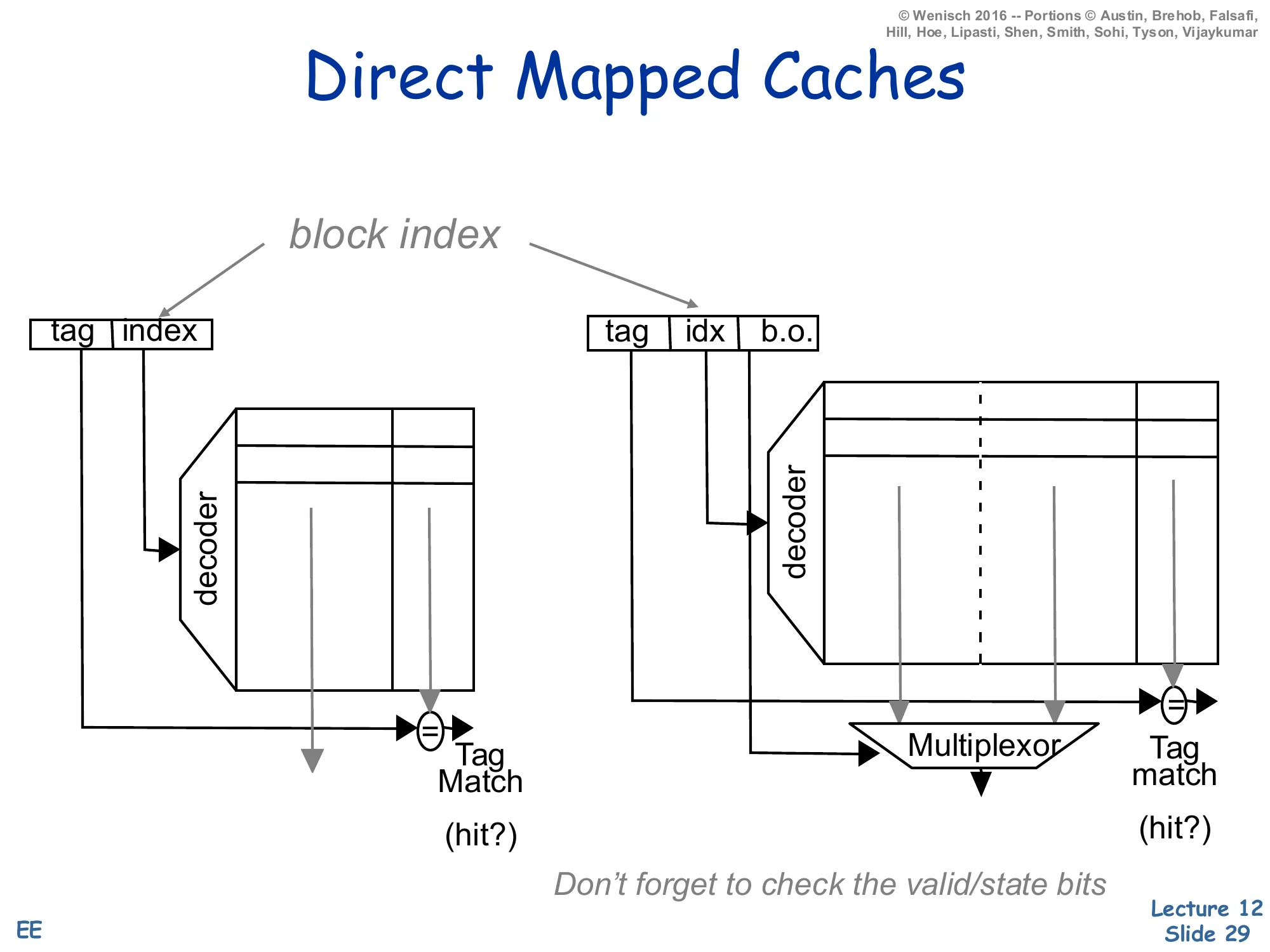
Direct Mapped Caches

Address decomposition: tag | index (1-byte block) or tag | idx | b.o. (multi-byte block).

Left: small direct-mapped cache, decoder selects a single row, tag-match comparator outputs hit?

Right: same with a multi-word block — block-offset (b.o.) drives a multiplexor that selects which word in the matched line is returned.

Don’t forget to check the valid/state bits.

A direct-mapped cache splits the address into three fields: high-order tag, middle index (selects the unique frame), low-order block offset (selects the byte/word within the line). The diagram shows the two-stage path: the decoder uses the index to fire one row of the SRAM, the row’s tag is compared with the address-tag (one comparator, no mux), and AND-ing match × valid produces the hit signal. With multi-word blocks the same row is read out in parallel and a block-offset mux selects which word the CPU asked for. This is the simplest cache imaginable — one comparator, one mux, no replacement policy needed because a block has exactly one place to live. The cost of the simplicity is conflict misses when two heavily-used addresses share an index. The slide’s reminder don’t forget the valid/state bits matters because a tag match alone isn’t sufficient: the frame might be storing a stale or unallocated tag that happens to match by coincidence after reset.

Fully Associative Cache

Slide 30

Show slide text

Fully Associative Cache

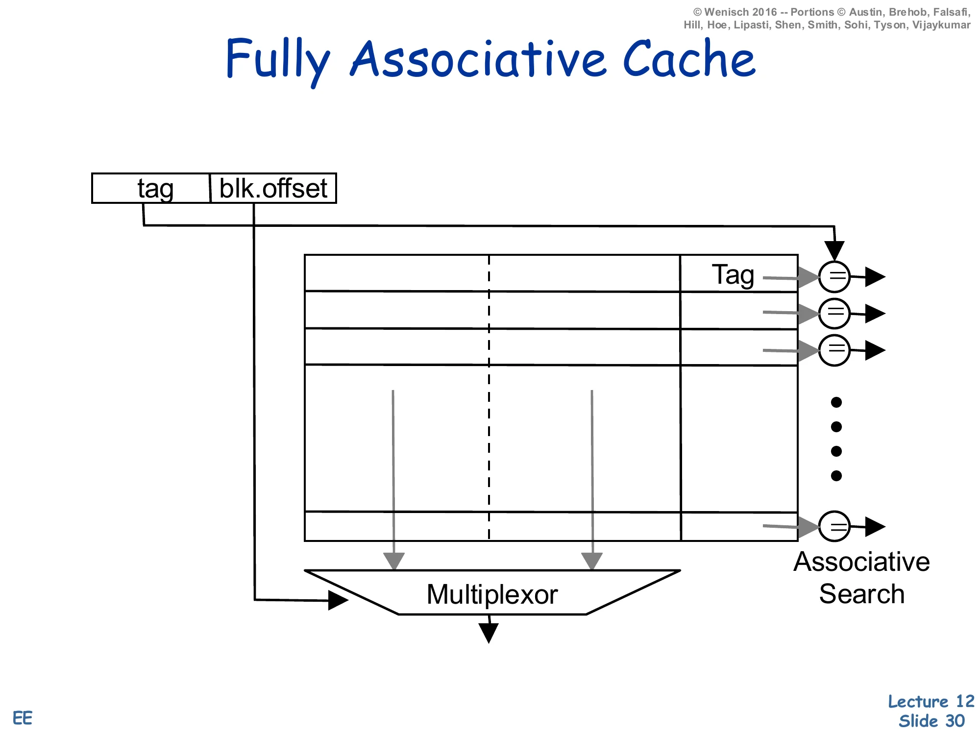
Address decomposition: tag | blk.offset (no index field).

Every frame in the cache holds (tag, data); a comparator on every row checks the incoming tag against the stored tag in parallel. Associative search. The matching row’s data is muxed to the output by the block offset.

Without an index field the address splits into just tag and block offset: every frame in the cache is a potential home for the block, so the lookup must compare the incoming tag against every stored tag in parallel — an associative search. This is exactly the structure of a TLB or a small victim cache. The hardware cost is one comparator per frame plus a wide priority encoder/mux that selects the matching row’s data; this scales as O($N$) in both area and power, which is why fully associative caches are limited to small structures (~tens to a few hundred entries). The benefit is zero conflict misses — any block can live anywhere, so a hot pair of addresses can co-reside no matter how their bits collide. A useful mental model: fully associative is set-associative with $\#\text{sets}=1$, just as direct-mapped is set-associative with associativity $a=1$.

N-Way Set Associative Cache

Slide 31

Show slide text

N-Way Set Associative Cache

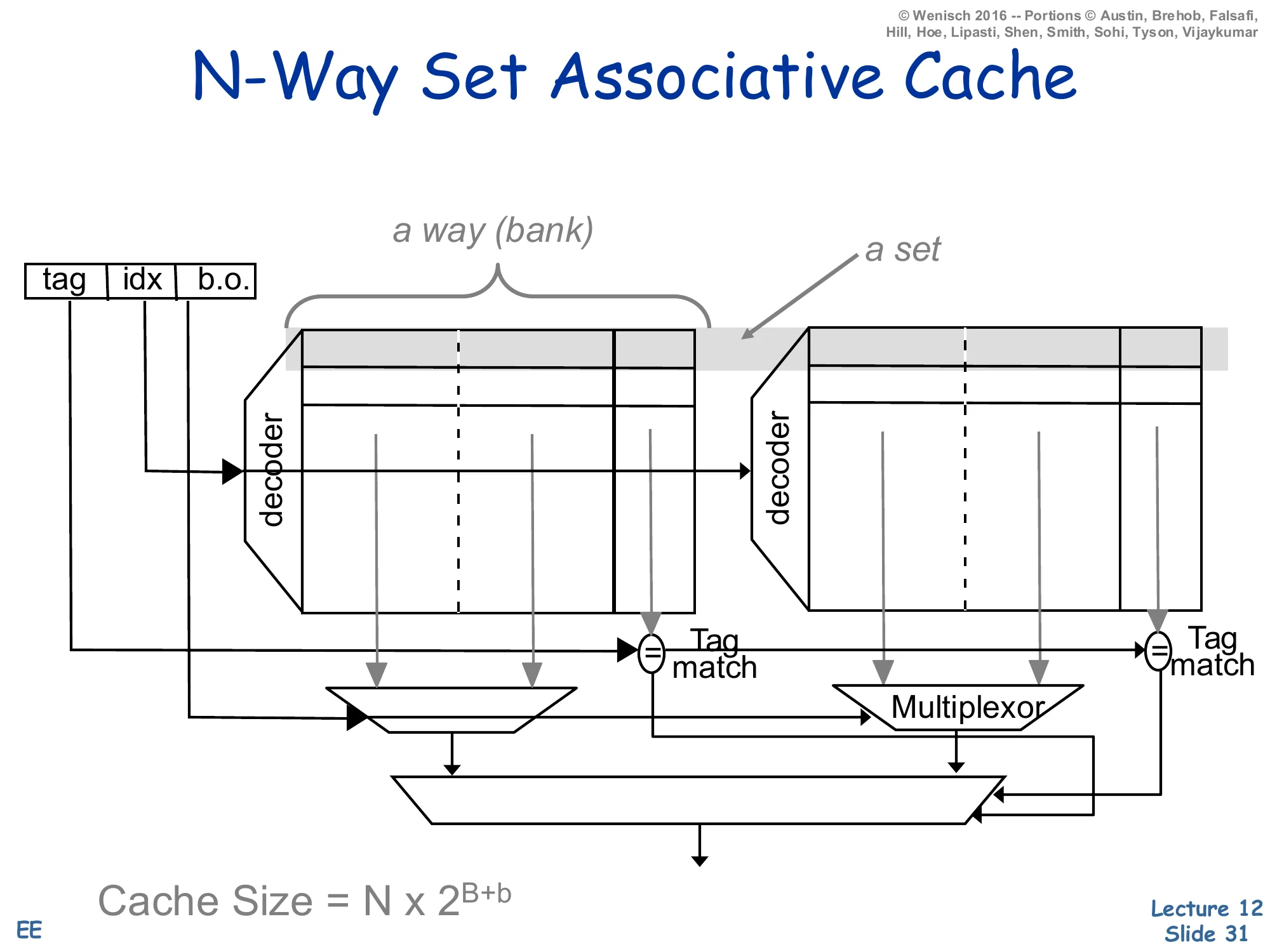
Address: tag | idx | b.o.

Two banks (a way) each indexed by idx. The set is the row across both ways. Each way has its own tag comparator; tag-match outputs feed a mux that selects which way’s data wins.

$\text{Cache Size} = N \times 2^{B+b}$

where $N$ = associativity, $2^B$ = number of sets, $2^b$ = bytes per block.

An $N$-way set-associative cache is the engineering compromise: $N$ parallel direct-mapped banks (called ways), each of $2^B$ rows of $2^b$-byte blocks. The address index selects a row across all ways simultaneously — that row, viewed across all ways, is the set. Each way’s tag is compared with the incoming tag in parallel, producing $N$ hit signals (at most one is true if the cache is consistent), and the set’s data is muxed to the output by the winning hit signal. Total capacity is $C = N \times 2^B \times 2^b$. Compared to fully associative the cost drops from $O(\#\text{frames})$ comparators to $O(N)$ — typically 2, 4, or 8 — and the index field localizes the search to one set instead of the whole cache. Compared to direct-mapped the conflict-miss rate drops sharply at the cost of the $N$-input data mux on the read path. This is the structure used by essentially every modern data cache.

Example: a=2, C=1kB, b=4B, word-size=2B

Slide 32

Show slide text

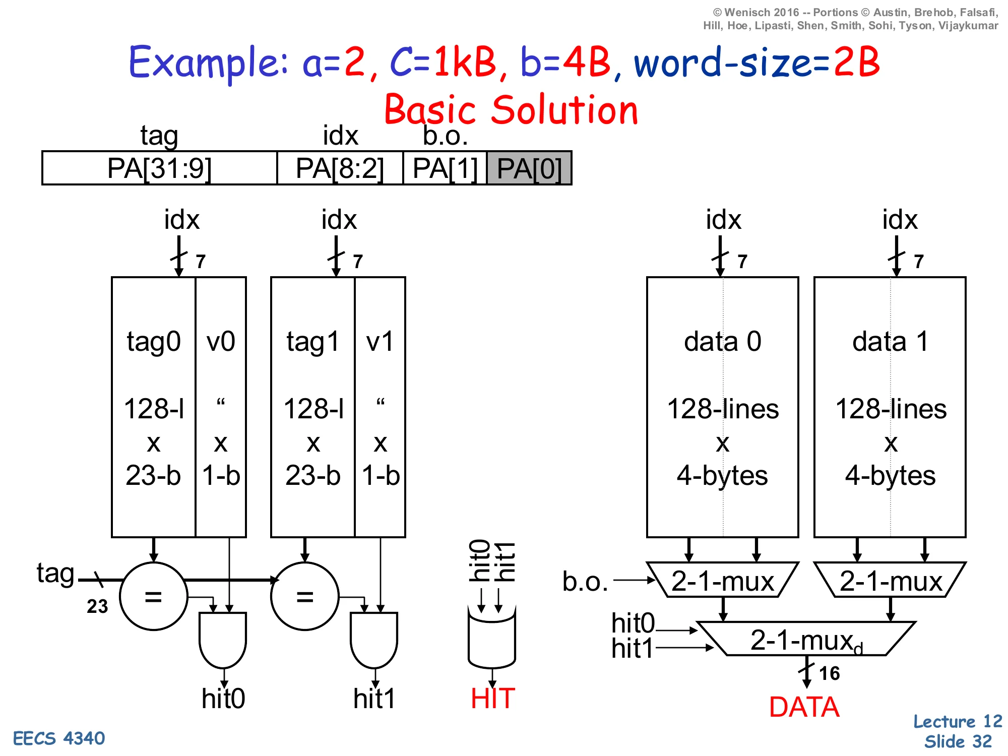
Example: $a=2$, $C=1\text{kB}$, $b=4\text{B}$, word-size=$2\text{B}$ — Basic Solution

Address fields (PA = physical address, 32 bits):

• tag = PA[31:9] (23 bits)
• idx = PA[8:2] (7 bits, $2^7 = 128$ sets)
• b.o. = PA[1] (1 bit selects which word in 4B block)
• PA[0] is the byte-in-word offset (greyed)

Tag arrays: two banks tag0|v0 and tag1|v1, each $128 \times (23\text{-bit tag} + 1\text{-bit valid})$.

Data arrays: two banks data 0, data 1, each $128 \times 4\text{ bytes}$.

Per access: drive idx[6:0] into all four arrays in parallel. Each tag bank produces a hit (hit0, hit1); HIT = hit0 OR hit1. Each data bank’s 4-byte row feeds a 2:1 b.o. mux to pick the requested 16-bit word, then a 2:1 mux selects the winning way’s word into DATA.

This worked example is the canonical “how do I size the address fields?” exercise. Capacity $C = 1024$ B, block $b = 4$ B, associativity $a = 2$. Number of sets $= C / (a \times b) = 1024 / 8 = 128 = 2^7$, so the index is 7 bits. Block-offset is $\log_2(b) = 2$ bits, but with a 2-byte word size the cache returns a word at a time, so only PA[1] selects which 2-byte word in the block; PA[0] is greyed because it is the byte-within-word that the load/store unit handles separately. The remaining $32 - 7 - 2 = 23$ bits are the tag. Storage cost per way: 128 rows × (23 + 1) tag-bits + 128 rows × 32 data-bits, doubled for two ways. The diagram shows all four SRAM banks driven by the same index in parallel, each tag bank’s compare-and-AND-with-valid producing hit0/hit1, and the data path using two 2:1 muxes — first the block-offset mux per-way to pick a word, then a way-select mux driven by the hit signals to choose which way’s data is returned. This style of derivation is testable: any cache problem with $C, b, a, \text{addr-width}$ given will reduce to the same arithmetic.

Another Example: AMD Opteron

Slide 33

Show slide text

Another Example: AMD Opteron

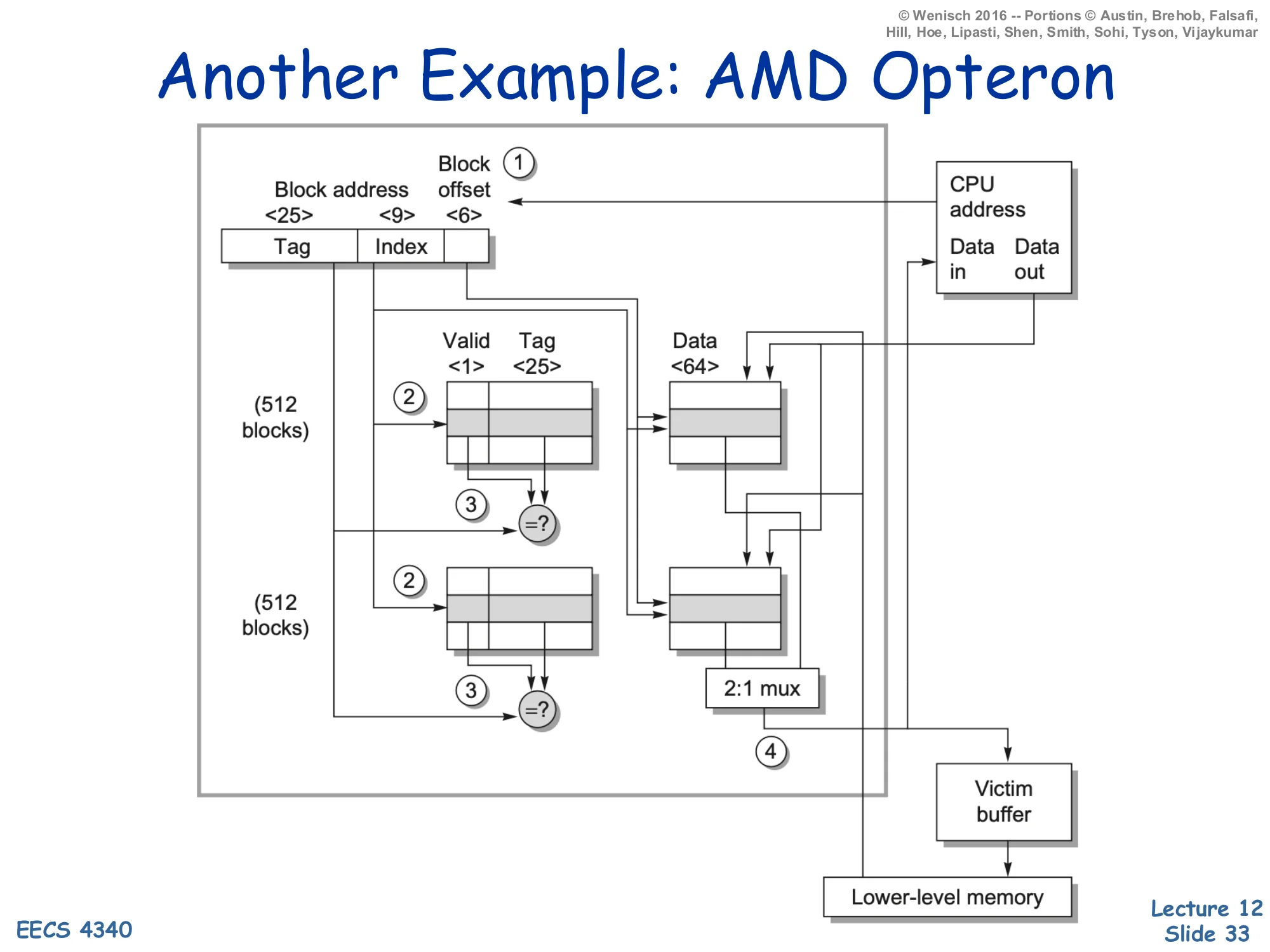
A 2-way set-associative cache, $b = 64$ B (block-offset 6 bits), $\#\text{sets} = 512$ (index 9 bits), tag = 25 bits, valid = 1 bit, data = 64 B per frame.

Annotated dataflow (1)–(4):

1. CPU presents address; split into tag, index, block-offset.
2. Index drives both tag arrays (512 entries each) and both data arrays.
3. Compare each way’s tag against the address-tag → hit signals; in parallel, both ways’ data feed a 2:1 mux.
4. On a hit the muxed word is returned to the CPU; on a miss the block is fetched from lower-level memory and any displaced dirty block is staged in the victim buffer before being written back.

The AMD Opteron L1 (one of the textbook reference designs) is a 64 KB 2-way set-associative cache with 64 B blocks. Walking the math: $\#\text{sets} = C / (a \cdot b) = 65536 / 128 = 512 = 2^9$ → 9-bit index; block-offset $= \log_2 64 = 6$ bits; tag $= 40 - 9 - 6 = 25$ bits (40-bit physical address). The diagram annotates the four steps of an access: address split (1), parallel tag and data lookup (2), tag-compare and data mux (3), and either CPU return or miss handling with a victim buffer (4). The victim buffer (Jouppi’s classic structure, the topic of one of this lecture’s recommended readings) holds recently evicted blocks for a few cycles; if a near-future access misses the L1 but hits in the victim buffer, the evicted block can be restored without going to L2. This is a cheap fix for the conflict-miss weakness of low-associativity caches like this 2-way design — and exactly the small fully-associative cache in the Jouppi paper title.

Associative Block Replacement

Slide 34

Show slide text

Associative Block Replacement

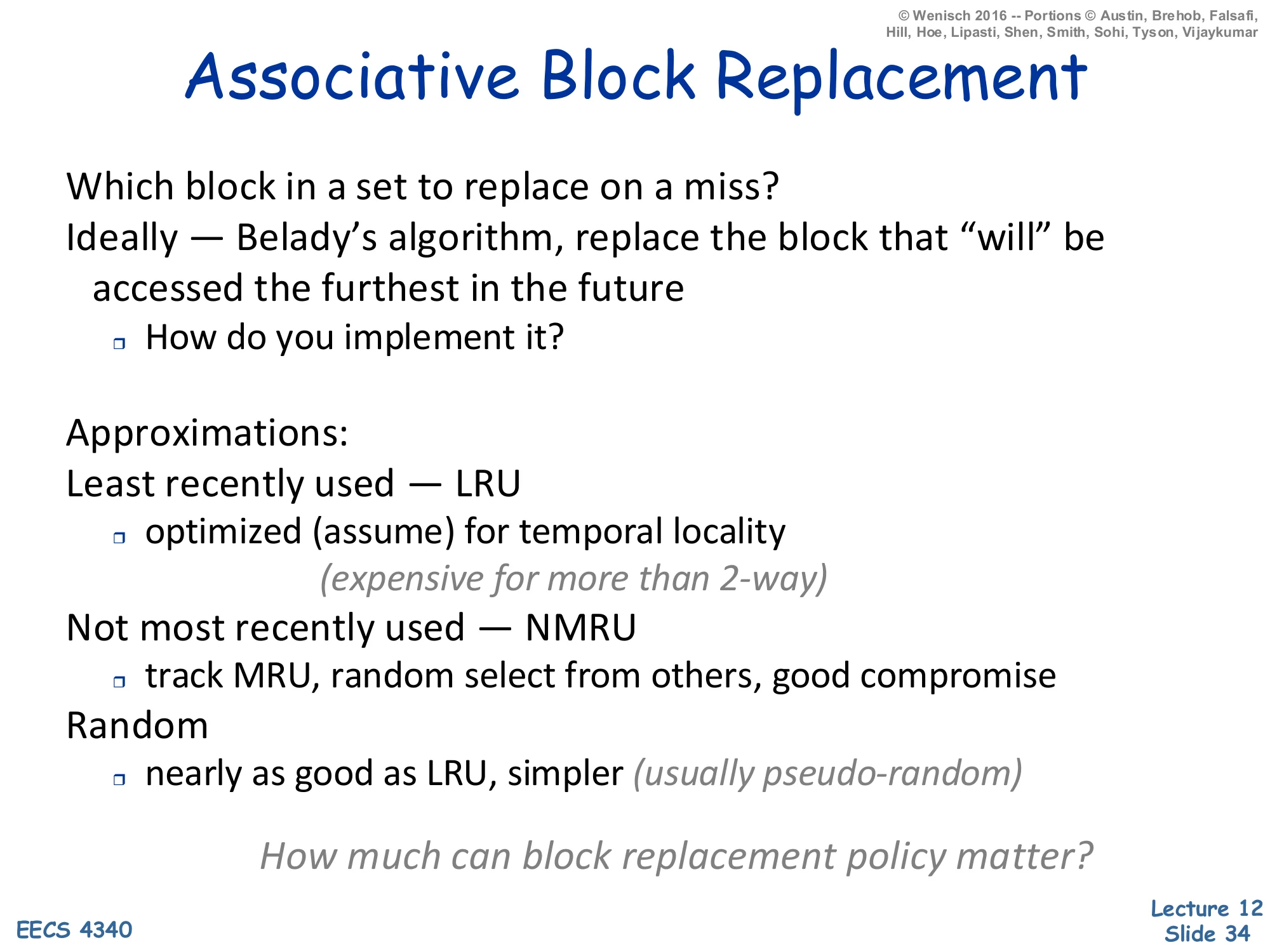
Which block in a set to replace on a miss?

Ideally — Belady’s algorithm: replace the block that “will” be accessed the furthest in the future.

• How do you implement it?

Approximations:

• Least recently used — LRU
  • optimized (assume) for temporal locality
  • (expensive for more than 2-way)
• Not most recently used — NMRU
  • track MRU, random select from others, good compromise
• Random
  • nearly as good as LRU, simpler (usually pseudo-random)

How much can block replacement policy matter?

Once a set is full, the cache must pick a victim. The optimum, Belady’s algorithm (also called OPT or MIN), evicts the block whose next reference is furthest in the future — but that requires omniscience, so it’s only a benchmark. Real implementations approximate. LRU (least recently used) tracks per-set access ordering and evicts the oldest; for 2-way it’s one age bit per set, but for $N$-way the bookkeeping grows as $\log_2(N!)$ bits per set and the update logic on every hit is non-trivial — by 8-way most designs stop being strictly LRU. NMRU tracks only the most-recently-used way and picks a random victim from the other $N-1$ — a single bit per set captures the bulk of LRU’s benefit. Random (pseudo-random) replacement is even simpler and is empirically only a few percent worse than LRU on most workloads. The trailing question on the slide is the practical one: replacement policy matters less than $C$, $b$, or $a$ — you should size the cache and tune associativity first, then pick the simplest policy that hits target hit-rate. By contrast, exotic policies like RRIP and LIRS exist precisely for last-level caches where conventional policies thrash.

Write Policies

Slide 35

Show slide text

Write Policies

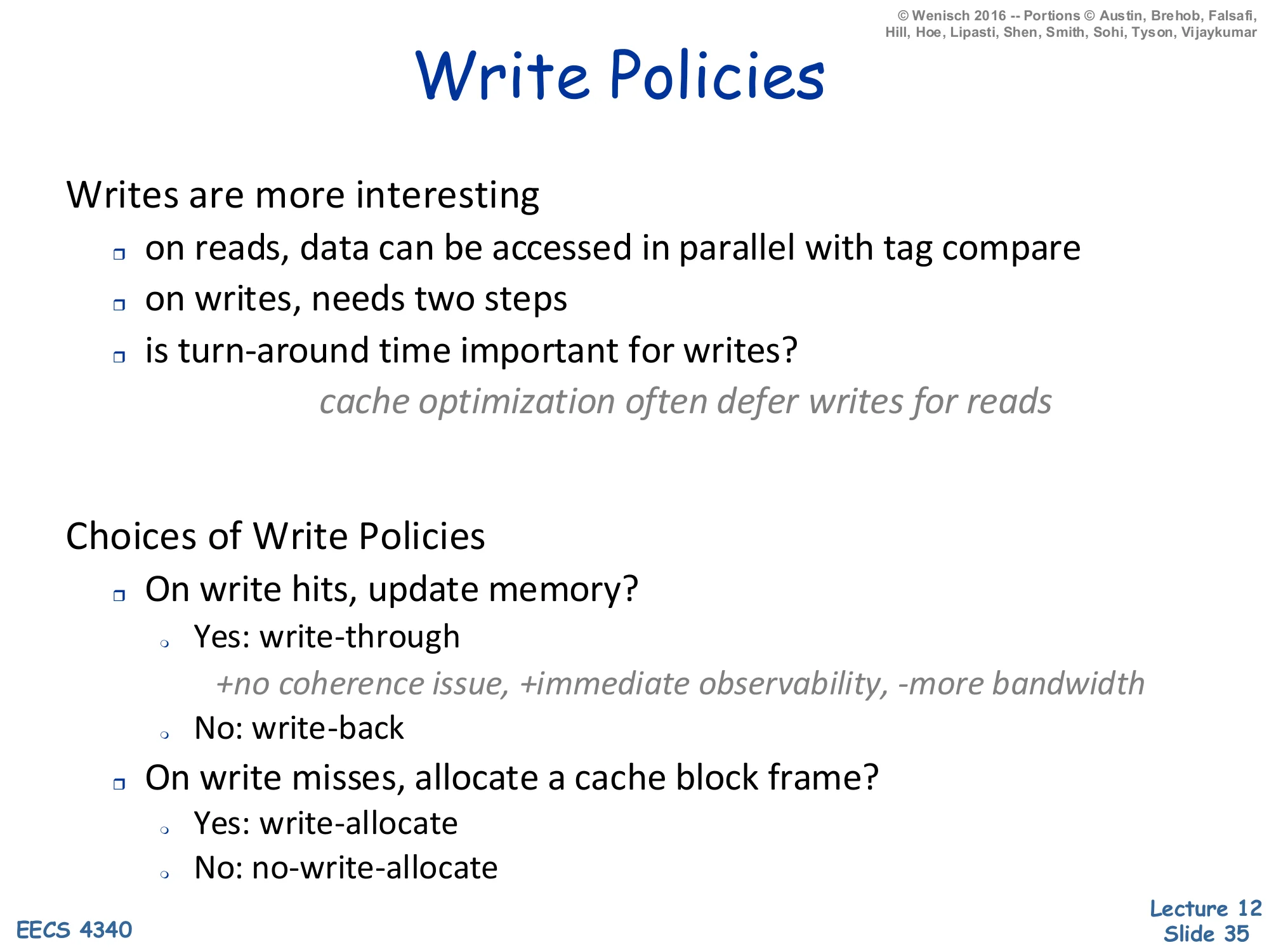
Writes are more interesting

• on reads, data can be accessed in parallel with tag compare
• on writes, needs two steps
• is turn-around time important for writes? cache optimization often defers writes for reads

Choices of Write Policies

• On write hits, update memory?
  • Yes: write-through (+no coherence issue, +immediate observability, −more bandwidth)
  • No: write-back
• On write misses, allocate a cache block frame?
  • Yes: write-allocate
  • No: no-write-allocate

Reads and writes are fundamentally asymmetric in caches. On a read the data SRAM can be accessed in parallel with the tag-compare, and the result is squashed if the tag misses — speculative prefetch of data is free. On a write you must first check the tag (you can’t corrupt data on a wrong line) and then commit the write, so writes are serialized two-step operations. Architects use this asymmetry: caches buffer writes through store-buffers and writeback-buffers (slides 37–38) so that read latency stays on the critical path while writes happen in the background. Two orthogonal policies fall out. The hit policy — write-through (propagate every store to the next level) versus write-back (only update next level on dirty eviction) — trades simpler coherence and immediate observability against bandwidth. The miss policy — write-allocate (load the block on a write miss, then write) versus no-write-allocate (write directly to next level, don’t pollute the cache) — depends on whether subsequent reads are likely. Common pairings: write-through usually pairs with no-write-allocate (simple, low-bandwidth), write-back usually pairs with write-allocate (high hit rate on subsequent loads to the same block).

Write Policies (Cont.)

Slide 36

Show slide text

Write Policies (Cont.)

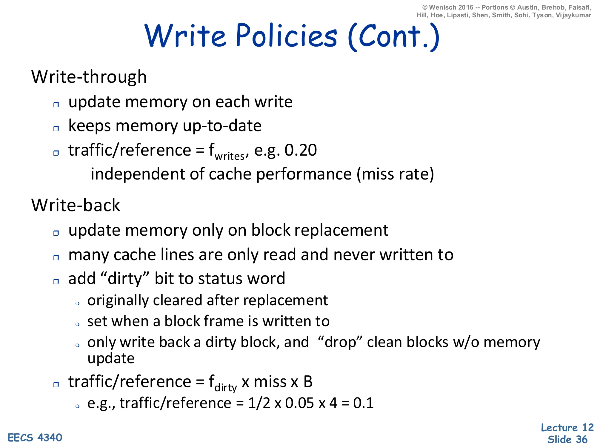
Write-through

• update memory on each write
• keeps memory up-to-date
• traffic/reference $= f_{\text{writes}}$, e.g. $0.20$
  • independent of cache performance (miss rate)

Write-back

• update memory only on block replacement
• many cache lines are only read and never written to
• add “dirty” bit to status word
  • originally cleared after replacement
  • set when a block frame is written to
  • only write back a dirty block, and “drop” clean blocks w/o memory update
• traffic/reference $= f_{\text{dirty}} \times \text{miss} \times B$
  • e.g., traffic/reference $= \tfrac{1}{2} \times 0.05 \times 4 = 0.1$

This slide quantifies the bandwidth difference between the two write policies. Write-through sends every store to the next level, so its traffic-per-reference equals the fraction of references that are stores — typically $f_{\text{writes}} \approx 0.2$ for SPEC-style integer code. Crucially, this traffic is independent of the miss rate: even a perfect cache with 0% misses still generates 20% write-traffic to the next level. Write-back tags every block with a dirty bit that is cleared on fill and set on the first write; only dirty blocks must be written back when evicted, and clean evictions can be silently dropped. The traffic-per-reference becomes $f_{\text{dirty}} \times \text{miss} \times B$ where $f_{\text{dirty}}$ is the fraction of evicted lines that are dirty (typically 1/2), miss is the cache miss rate (e.g., 5%), and $B$ is the size in transfer-unit bytes (here 4). The example arithmetic gives 0.1 — half the bandwidth of write-through. The cost of write-back is added complexity: a dirty bit per line, a writeback buffer to stage evictions, and harder coherence in multi-core systems because dirty data exists only in one cache. Modern designs uniformly use write-back at L1 and below.

Store Buffers

Slide 37

Show slide text

Store Buffers

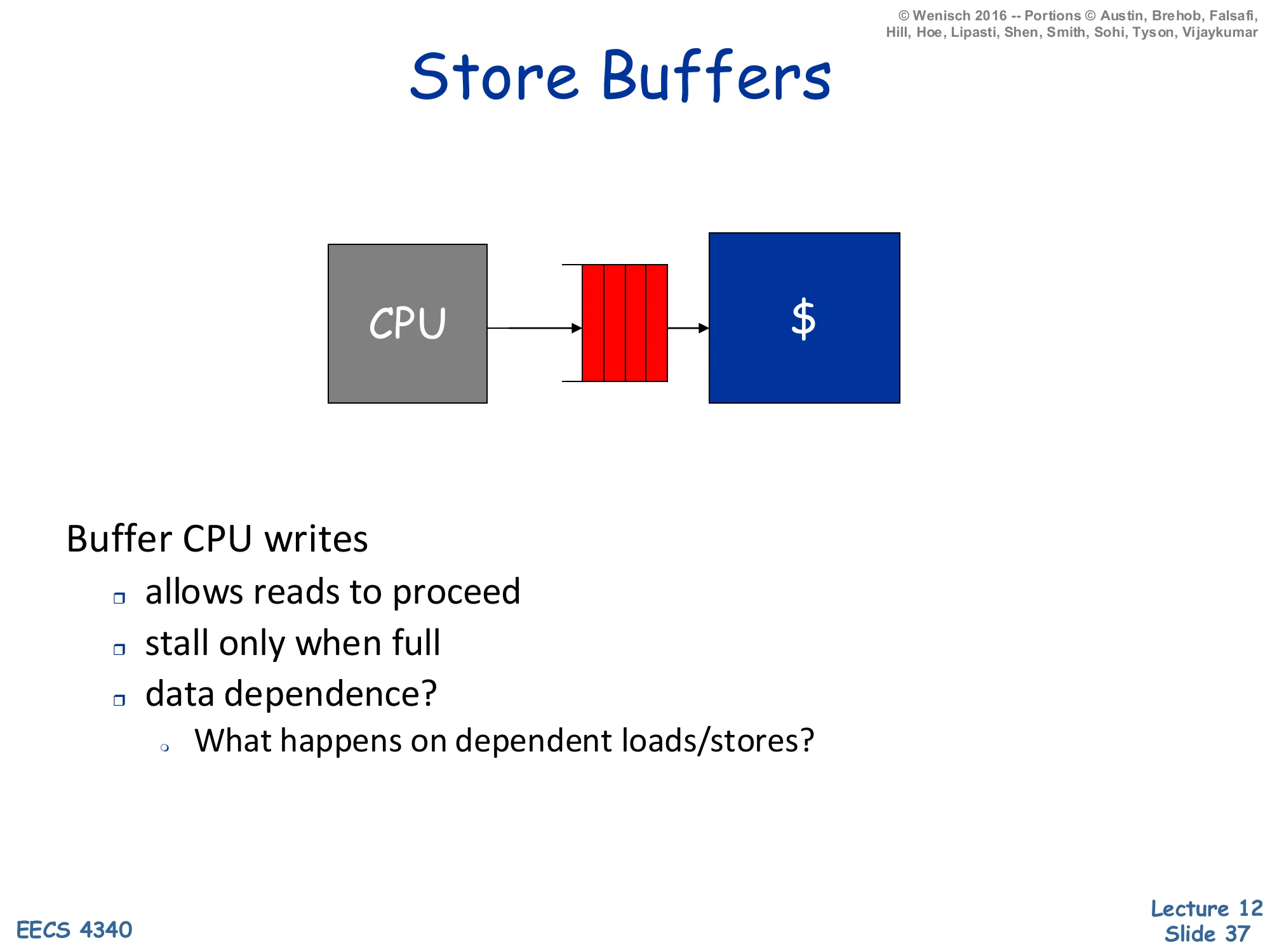
CPU → store buffer (red FIFO) → cache.

Buffer CPU writes

• allows reads to proceed
• stall only when full
• data dependence?
  • What happens on dependent loads/stores?

A store buffer sits between the pipeline’s commit stage and the L1 cache. Its job is to absorb the latency mismatch: stores are committed every cycle, but a write-through cache (or a write-back cache that needs a tag-check-then-write sequence) cannot absorb every store at full pipeline rate. By queueing committed stores in a small FIFO, the pipeline can fall through and let load-driven hits stay on the cache’s critical path; stores drain into the cache opportunistically when the cache is otherwise idle. The pipeline only stalls when the store buffer fills. The data-dependence question on the slide is the subtle part: a younger load that addresses the same byte as an older still-buffered store must forward the buffered value rather than read stale data from the cache. This is store-to-load forwarding, implemented by an associative search over the store buffer on every load — a major source of complexity in modern out-of-order pipelines, and the gateway to memory disambiguation which the lecture covers later.

Writeback Buffers

Slide 38

Show slide text

Writeback Buffers

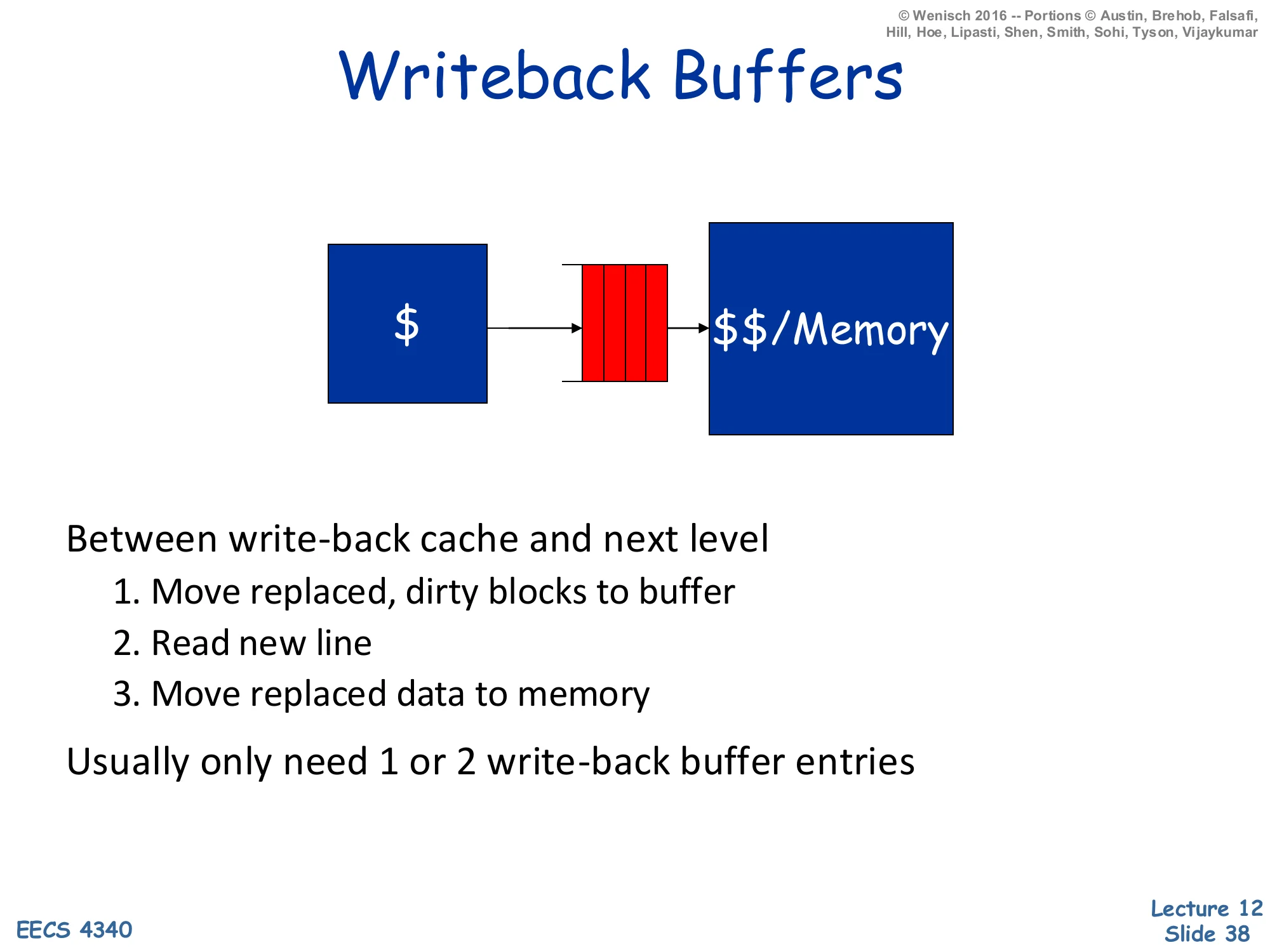
Cache → writeback buffer (red FIFO) → next-level cache or memory.

Between write-back cache and next level:

1. Move replaced, dirty blocks to buffer
2. Read new line
3. Move replaced data to memory

Usually only need 1 or 2 write-back buffer entries.

A writeback buffer (sometimes called a victim/eviction buffer in this context — distinct from Jouppi’s victim cache) sits between a write-back cache and the next level of the hierarchy. On a miss that requires evicting a dirty line, naive ordering would (1) write the dirty line back, then (2) read the new line — adding the writeback latency to the critical-path miss penalty. The writeback buffer breaks the dependency: (1) move the dirty line to the buffer in one cycle, (2) start the read of the new line immediately, and (3) drain the buffered dirty line to memory in the background while the new line returns. The CPU sees only one access latency rather than two. Because evictions are infrequent compared to fills, one or two buffer entries suffice; the buffer can drop to capacity-zero and merely stall on the rare back-to-back-evictions case. The downside is a small coherence wrinkle: a younger access to the same address as the buffered dirty line must forward from the buffer (similar logic to the store buffer on slide 37).

"Harvard" vs. "Princeton"

Slide 39

Show slide text

”Harvard” vs. “Princeton”

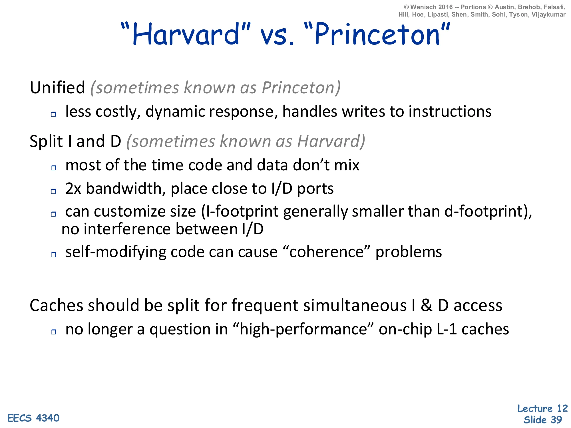
Unified (sometimes known as Princeton)

• less costly, dynamic response, handles writes to instructions

Split I and D (sometimes known as Harvard)

• most of the time code and data don’t mix
• 2× bandwidth, place close to I/D ports
• can customize size (I-footprint generally smaller than d-footprint), no interference between I/D
• self-modifying code can cause “coherence” problems

Caches should be split for frequent simultaneous I & D access — no longer a question in “high-performance” on-chip L-1 caches.

The Harvard vs. Princeton naming is historic: the original Harvard Mark I had separate physical paths for instructions and data, while the Princeton/von-Neumann architecture unified them. In a unified cache, instructions and data share one structure: simpler, dynamically allocates capacity to whichever stream is hotter, and trivially handles self-modifying code (a store-to-instruction goes to the same line that the fetch unit will read). In a split cache, the L1 instruction cache (L1-I) and L1 data cache (L1-D) are separate structures sitting next to their respective ports — the I-side near the fetch unit, the D-side near the load-store unit. The split organization gives 2× bandwidth (independent ports), eliminates I/D interference (a memcpy doesn’t evict the hot loop body), allows independent sizing (I-cache is usually smaller because instruction footprints are denser than data working sets), and shortens the wires from each port. The cost is self-modifying code coherence: a store hits L1-D, but the fetch unit reads L1-I — without explicit coherence the modified instruction is invisible. Modern x86 ISAs maintain self-modifying-code coherence in hardware via snoops; ISAs like ARM and RISC-V require explicit IC INVAL / fence.i instructions instead. The closing line says it all: at L1, on-chip, all modern high-performance designs are split.

Readings

Slide 40

Show slide text

Readings

For today:

• H & P Chapter 2.1, Appendix B.1, and B.2

For Wednesday:

• H & P Chapter 2.2, 2.3, and Appendix B.3
• Improving direct-mapped cache performance by the addition of a small fully-associative cache and prefetch buffers, https://dl.acm.org/doi/abs/10.1145/325096.325162

Announcements

Slide 41

Show slide text

Announcements

• Project #4
  • Due: 22-April-26
• Project meetings
  • Mondays and Wednesdays during my office hours

https://courseworks2.columbia.edu/courses/237081