L14 · Prefetching
L14 · Prefetching
Topic: memory · 46 pages
EECS 4340 Lecture 14 — Prefetching

Announcements

Show slide text
Announcements
- Project #4
- Due: 1-May-26
- Final project presentation
- May 4, 2026
- 8:40 to 9:50 AM
- 8 minutes per group, schedule on Courseworks
Readings

Show slide text
Readings
For today:
- A primer on hardware prefetching, https://doi.org/10.1007/978-3-031-01743-8
For next Monday:
- Appendix L, http://www.cs.yale.edu/homes/abhishek/abhishek-appendix-l.pdf
- Architectural and Operating System Support for Virtual Memory, https://doi.org/10.1007/978-3-031-01757-5
Recap: Advanced Caches
Multi-Level Cache Design
Show slide text
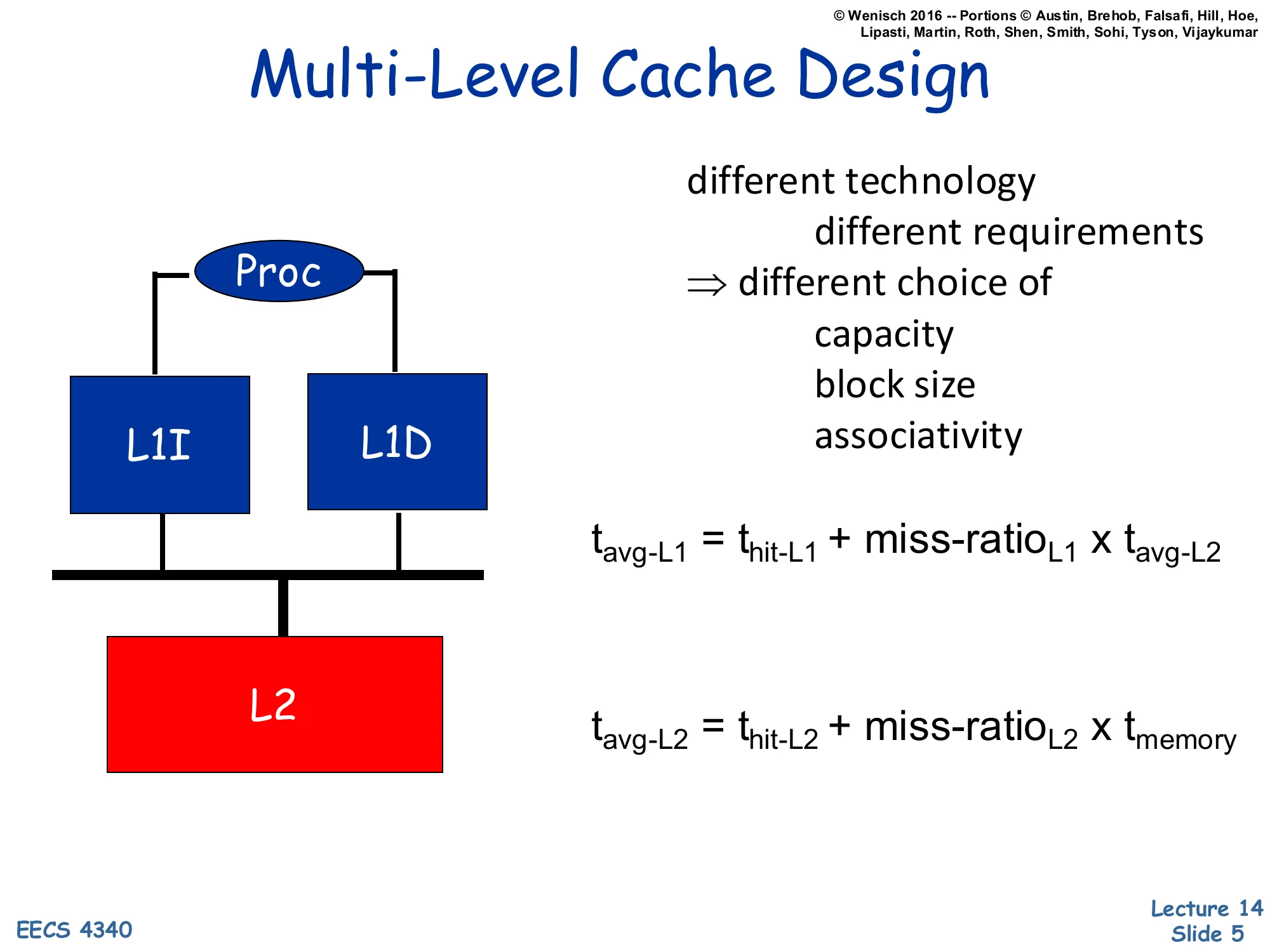
Multi-Level Cache Design
- Different technology, different requirements ⇒ different choice of
- capacity
- block size
- associativity
Proc → L1I, L1D → L2
tavg-L1=thit-L1+miss-ratioL1×tavg-L2
tavg-L2=thit-L2+miss-ratioL2×tmemory
A multi-level cache hierarchy lets each level be tuned independently for its role. The L1 caches sit on the critical path of the pipeline, so they are kept small and fast and are usually split into separate L1I and L1D arrays so instruction fetch and data access can proceed in parallel. The L2 backs both L1s, is much larger and slower, and acts mostly to filter accesses before main memory. Because requirements differ, the cache-block size, associativity, and capacity may all differ between levels: a small L1 prefers low associativity for hit time while a larger L2 can afford more associativity to reduce conflict misses. The two equations on the slide are the recursive form of AMAT: the L1’s average access time depends on how often it misses and on the L2’s average access time, which itself depends on its miss rate and memory latency. Reading the equations bottom-up makes the design intuition concrete — a tiny improvement in L1 hit time compounds across every reference, while reducing the L2 miss rate is what saves you from paying the much larger main-memory penalty.
Non-blocking Caches
Show slide text
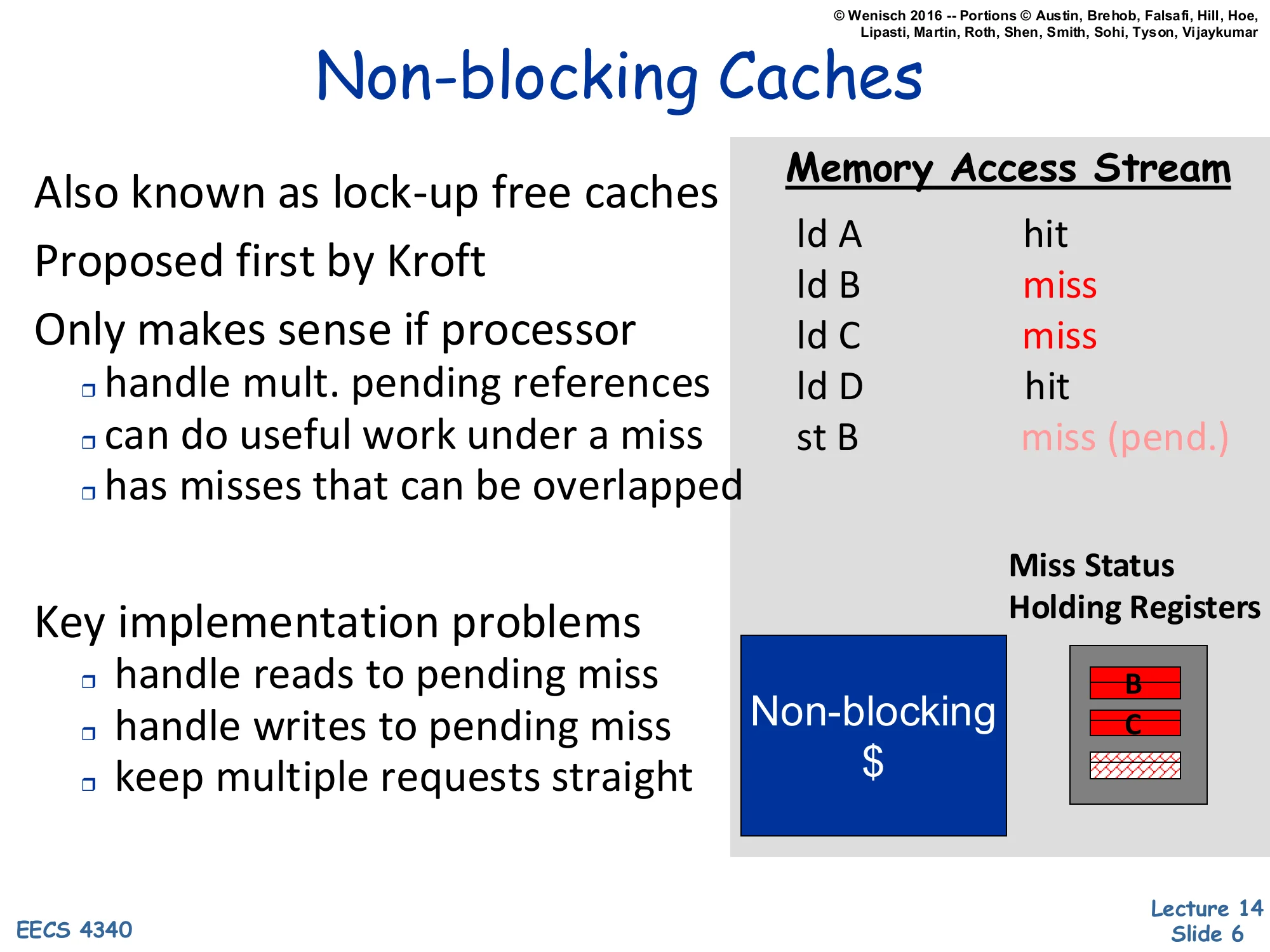
Non-blocking Caches
- Also known as lock-up free caches
- Proposed first by Kroft
- Only makes sense if processor
- handle mult. pending references
- can do useful work under a miss
- has misses that can be overlapped
- Key implementation problems
- handle reads to pending miss
- handle writes to pending miss
- keep multiple requests straight
Memory Access Stream
| Instruction | Status |
|---|---|
| ld A | hit |
| ld B | miss |
| ld C | miss |
| ld D | hit |
| st B | miss (pend.) |
Non-blocking $ → Miss Status Holding Registers (MSHRs) hold pending B, C.
A blocking cache stalls on every miss, which wastes any potential overlap between the miss latency and other useful work. A non-blocking (lock-up free) cache, originally proposed by Kroft, instead allows the processor to keep issuing references while one or more misses are outstanding. Each in-flight miss is tracked in a Miss Status Holding Register (MSHR) that records the address, the destination register or store buffer entry, and any subsequent accesses that hit the same line. When a later load to a still-pending line arrives (e.g. st B while B’s miss is in flight), the MSHR merges it instead of issuing a duplicate request. Non-blocking caches are only useful if the rest of the core can sustain in-flight memory operations: an out-of-order pipeline with a store buffer can do useful work under a miss, while an in-order machine that stalls on the next dependent instruction gains very little. The implementation challenges — handling reads and writes to a pending miss and keeping the request stream coherent — are exactly what make MSHR design subtle in practice.
Multi-Port Caches: True Multiporting
Show slide text
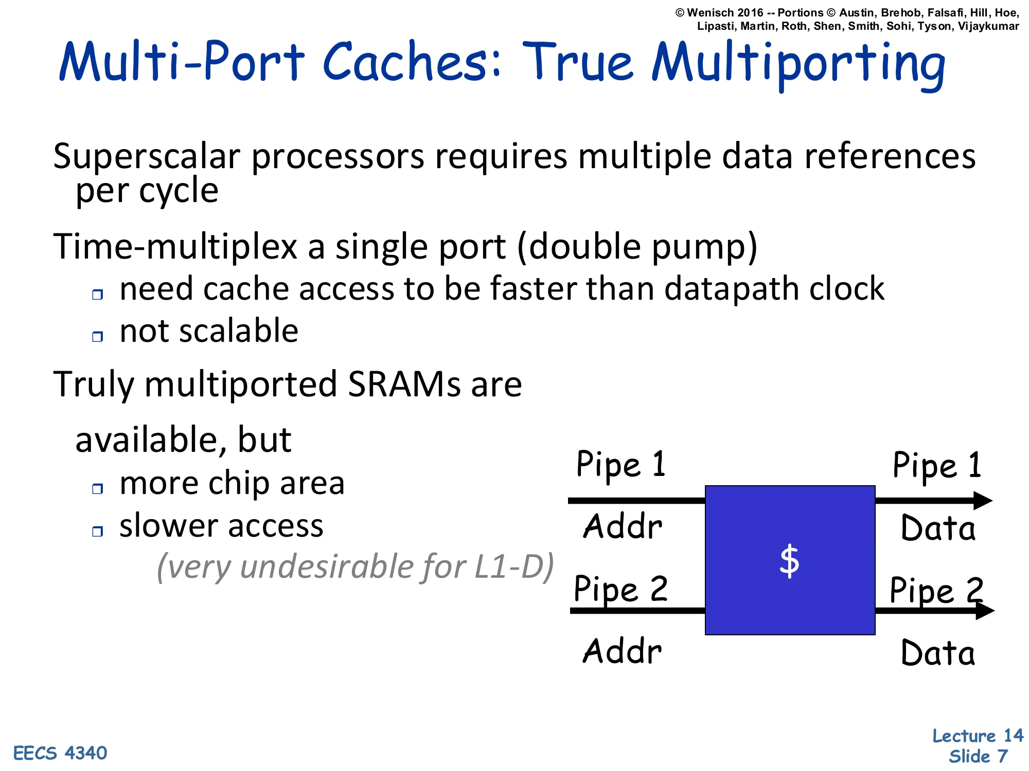
Multi-Port Caches: True Multiporting
- Superscalar processors require multiple data references per cycle
- Time-multiplex a single port (double pump)
- need cache access to be faster than datapath clock
- not scalable
- Truly multiported SRAMs are available, but
- more chip area
- slower access
- (very undesirable for L1-D)
Diagram: Pipe 1 (Addr → )→Data;Pipe2(Addr→) → Data.
A superscalar core can issue two or more memory operations per cycle, but the L1 data cache has a single SRAM array. There are three ways to support multiple accesses. First, double-pumping time-multiplexes one port at twice the clock — feasible only when the SRAM is fast enough relative to the datapath, and it does not scale beyond two accesses. Second, a truly multiported SRAM cell adds extra word-line and bit-line pairs per cell. That works for small structures like the register file but is undesirable for the L1-D because each extra port roughly doubles area and stretches access time, which directly hurts hit latency on the critical path. The third option — banking — appears on the next slide. The key takeaway is that the L1-D is so latency-sensitive that architects rarely accept the area and timing cost of full multiporting; they instead exploit the fact that simultaneous accesses usually fall in different parts of the address space, which a banked design handles cheaply.
Multi-Banking (Interleaving) Caches
Show slide text
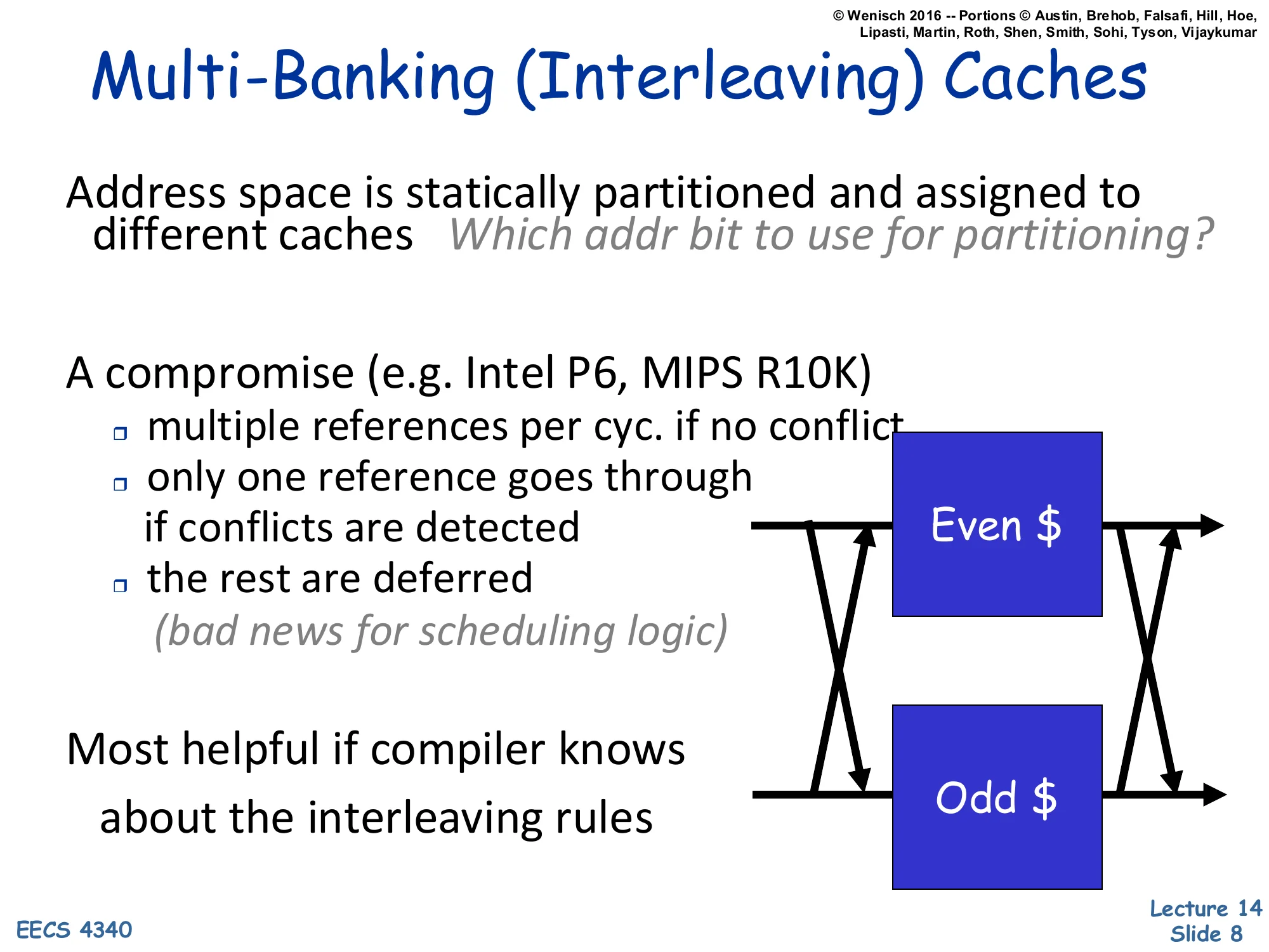
Multi-Banking (Interleaving) Caches
- Address space is statically partitioned and assigned to different caches. Which addr bit to use for partitioning?
- A compromise (e.g. Intel P6, MIPS R10K)
- multiple references per cyc. if no conflict
- only one reference goes through if conflicts are detected
- the rest are deferred (bad news for scheduling logic)
- Most helpful if compiler knows about the interleaving rules
Diagram: crossbar between two pipes and Even-/Odd− banks.
Multi-banking sidesteps the cost of true multiporting by splitting the cache into independent SRAM banks, each with one port, and statically partitioning addresses across banks (most often by a few low-order line-address bits so adjacent lines hit different banks). When two simultaneous accesses target different banks they both proceed in parallel; when they target the same bank a bank conflict is detected and one access is deferred. The Intel P6 and MIPS R10K used this scheme as a pragmatic compromise — it gives near-multiport throughput at roughly single-port area but pushes complexity into the issue/scheduling logic, which must handle the deferred reference, replay it next cycle, and avoid deadlock. The choice of which address bits select the bank matters: too high a bit and consecutive array accesses all land in the same bank; too low and you split a single line across banks. Compiler-aware code (e.g. unrolled loops with stride padding) can deliberately steer simultaneous accesses to different banks.
Multi-porting vs. Multibanking
Show slide text
Multi-porting vs. Multibanking
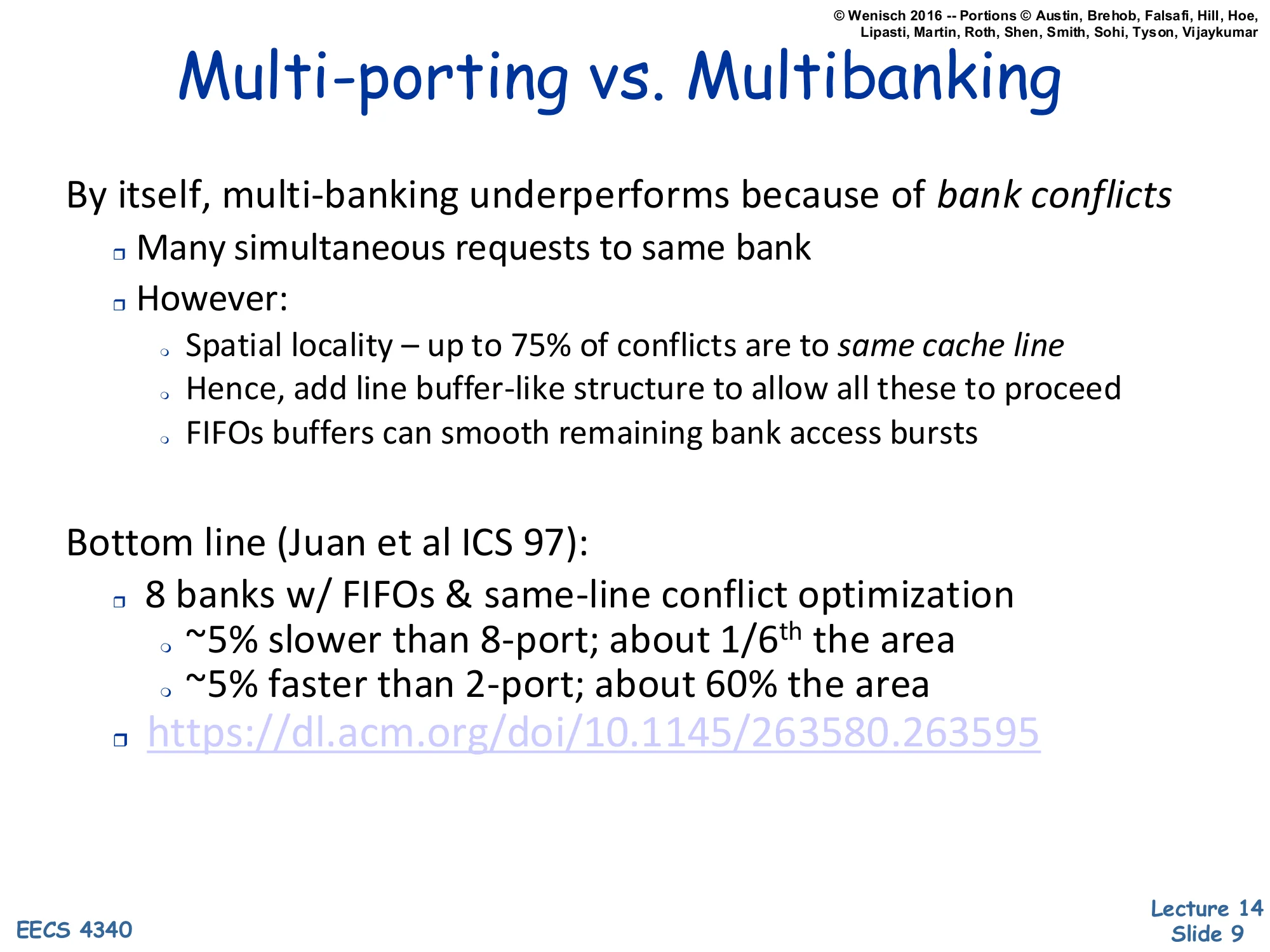
- By itself, multi-banking underperforms because of bank conflicts
- Many simultaneous requests to same bank
- However:
- Spatial locality — up to 75% of conflicts are to same cache line
- Hence, add line buffer-like structure to allow all these to proceed
- FIFOs buffers can smooth remaining bank access bursts
- Bottom line (Juan et al ICS ‘97):
- 8 banks w/ FIFOs & same-line conflict optimization
- ~5% slower than 8-port; about 1/6th the area
- ~5% faster than 2-port; about 60% the area
- https://dl.acm.org/doi/10.1145/263580.263595
- 8 banks w/ FIFOs & same-line conflict optimization
Pure multi-banking can stumble on bank conflicts, but two cheap optimizations close most of the gap with true multiporting. The first observation is that up to ~75% of bank conflicts are between accesses to the same cache line (a load and store to neighboring words, or two loads from the same line). A small line buffer in front of each bank lets all of these accesses share one SRAM read and proceed in the same cycle. The second optimization is per-bank FIFO request queues, which absorb temporary bank-access bursts so a brief hot spot does not cascade into a stall. Juan et al. (ICS ‘97) reported that an 8-bank cache with line-conflict bypass and FIFOs is only ~5% slower than a true 8-port SRAM at about one-sixth the area, and is actually ~5% faster than a 2-port SRAM at 60% of its area. The lesson is that exploiting cache-line-level spatial locality can recover most of the throughput a true multi-port would deliver, at a fraction of the area and with much shorter access time.
Non-Uniform Cache Architecture
Show slide text
Non-Uniform Cache Architecture
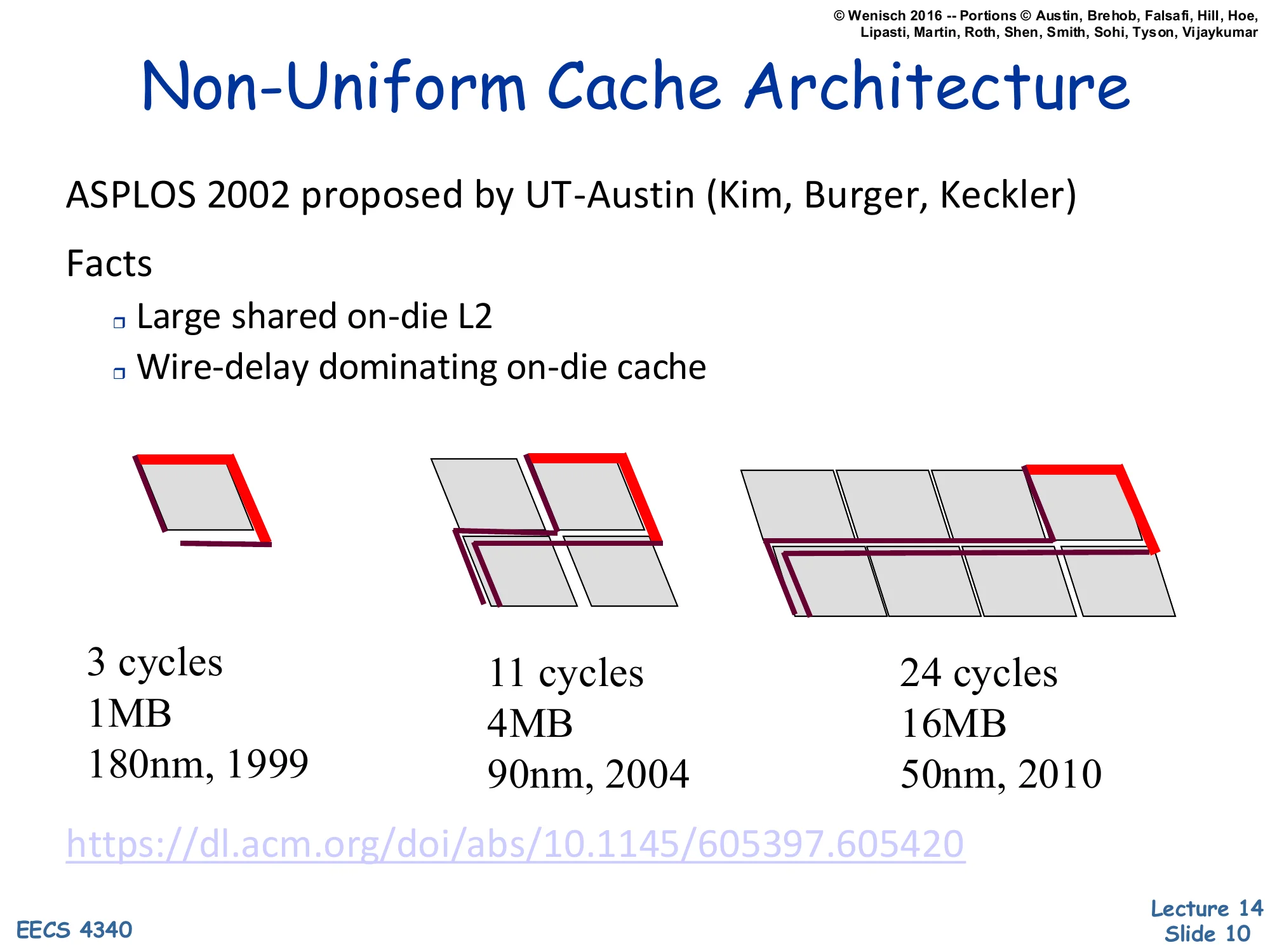
- ASPLOS 2002 proposed by UT-Austin (Kim, Burger, Keckler)
- Facts
- Large shared on-die L2
- Wire-delay dominating on-die cache
| Tile size | Cache size | Process / year |
|---|---|---|
| 3 cycles | 1 MB | 180 nm, 1999 |
| 11 cycles | 4 MB | 90 nm, 2004 |
| 24 cycles | 16 MB | 50 nm, 2010 |
As on-chip caches grew into multi-megabyte arrays, wire delay rather than SRAM access time started to dominate. Every doubling of capacity moves the farthest sub-array further from the cache controller, so a single uniform-latency design has to be paced to the worst-case corner. The data on the slide make the trend concrete: a 1 MB cache in 180 nm takes 3 cycles, but a 16 MB cache in 50 nm takes 24 cycles even though transistors got faster. The Non-Uniform Cache Architecture (NUCA) proposal from UT-Austin (Kim, Burger, Keckler, ASPLOS ‘02) accepts this reality: split the L2 into a grid of small banks each with its own access latency, and let nearby banks be reachable in a few cycles while far banks pay extra. Accesses then complete in different cycle counts depending on which bank holds the requested line. The next slide covers the two flavors — Static (S-NUCA), where each address has a fixed home bank, and Dynamic (D-NUCA), where lines migrate toward the requesting core.
Static and Dynamic NUCA
Show slide text
Static and Dynamic NUCA
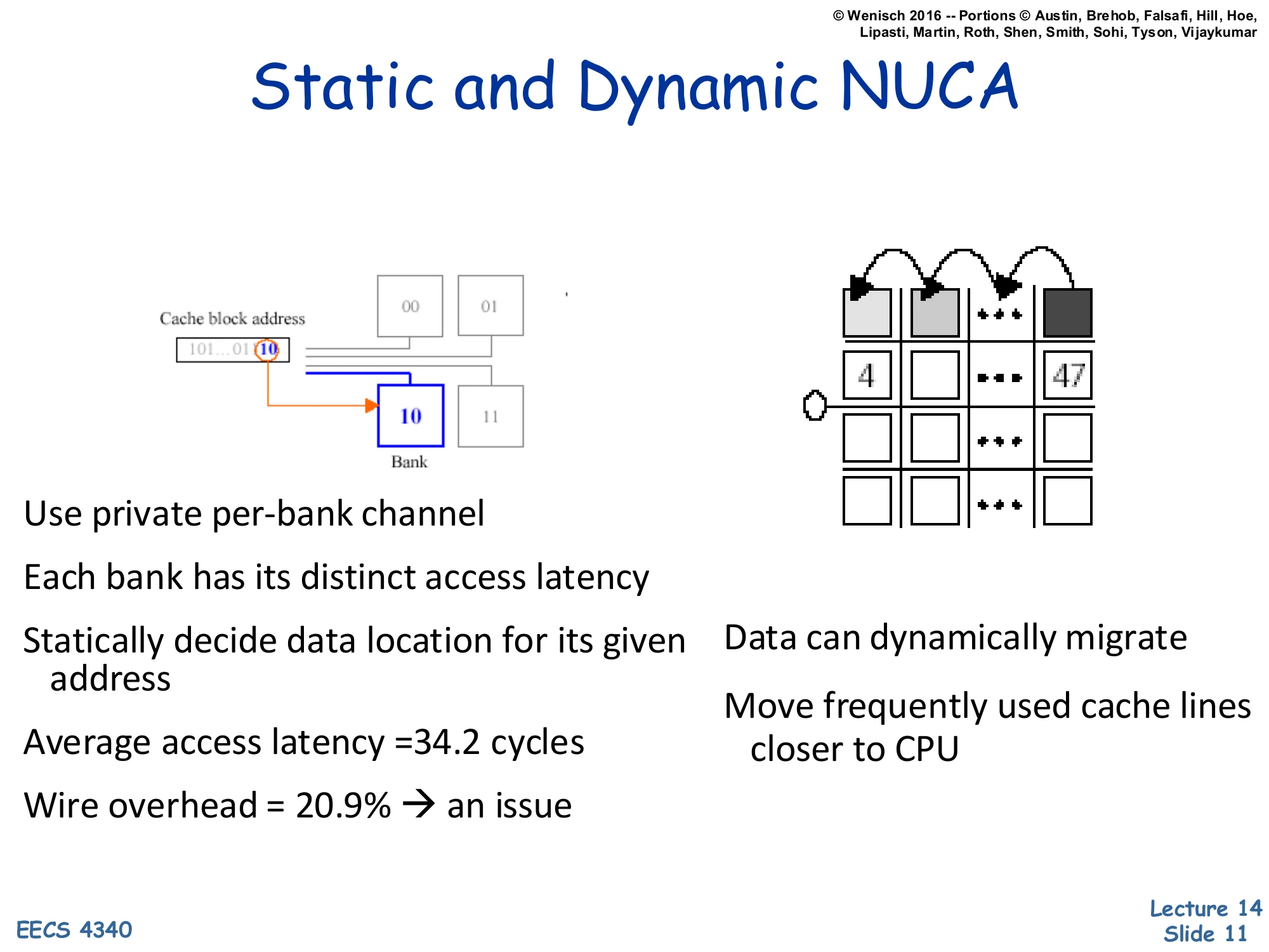
- Use private per-bank channel
- Each bank has its distinct access latency
- Statically decide data location for its given address
- Average access latency = 34.2 cycles
- Wire overhead = 20.9% → an issue
- Data can dynamically migrate
- Move frequently used cache lines closer to CPU
Static NUCA (S-NUCA) maps each cache block to one fixed bank chosen by some address bits — like multi-banking, but with a private channel per bank so bank latency varies with physical distance. The control logic is simple (a regular address-to-bank function), but the average access time is fixed at the mean over all banks: the slide quotes 34.2 cycles average with about 21% of the access budget consumed by wire delay. Dynamic NUCA (D-NUCA) addresses this inefficiency by migrating hot lines toward the requesting core: a frequently used line is gradually promoted from a far bank to a near bank by swapping entries on each access, so the steady-state hit latency for hot data drops well below the static average. The cost is higher control complexity (a search policy across banks, an LRU-like promotion rule, and care to avoid duplication or starvation). The diagram on the right shows the migration sequence — a line accessed via the bottom-left port hops up the column toward the requesting tile, displacing a colder line each step.
Prefetching

The Memory Wall
Show slide text
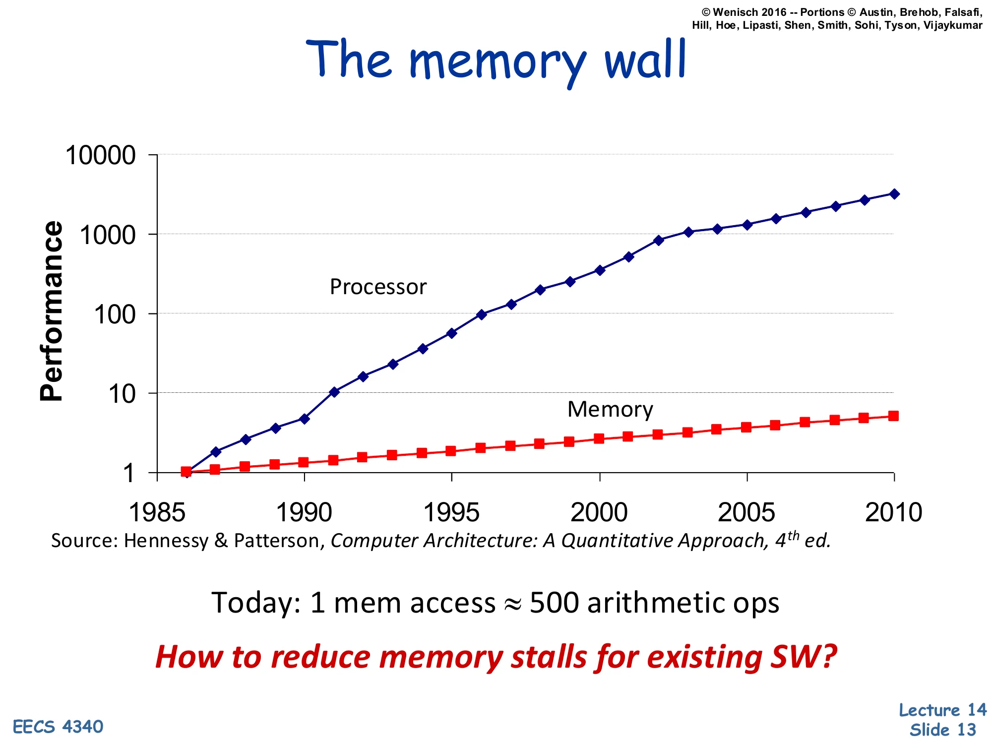
The Memory Wall
Processor performance grew far faster than DRAM performance from 1985 to 2010 (log scale plot, Hennessy & Patterson 4th ed.).
Today: 1 mem access ≈ 500 arithmetic ops.
How to reduce memory stalls for existing SW?
The memory wall is the gap between processor and memory performance growth. From 1985 to 2010 processor performance climbed roughly three orders of magnitude on the log-scale plot while DRAM access time barely improved by a single order — so today a single off-chip memory access costs roughly 500 arithmetic operations. Two architectural reactions to this gap (covered next) are insufficient on their own: bigger cache hierarchies have diminishing returns and don’t help cold or coherence misses, and out-of-order execution can only hide as much latency as fits in the reorder buffer. The motivating question for the rest of the lecture — how do we cut memory stalls for existing software, without rewriting it — is exactly what prefetching tries to answer: speculatively fetch lines before the processor demands them, so what would have been a long-latency miss becomes a short hit.
Conventional Approach #1: Avoid Main Memory Accesses
Show slide text
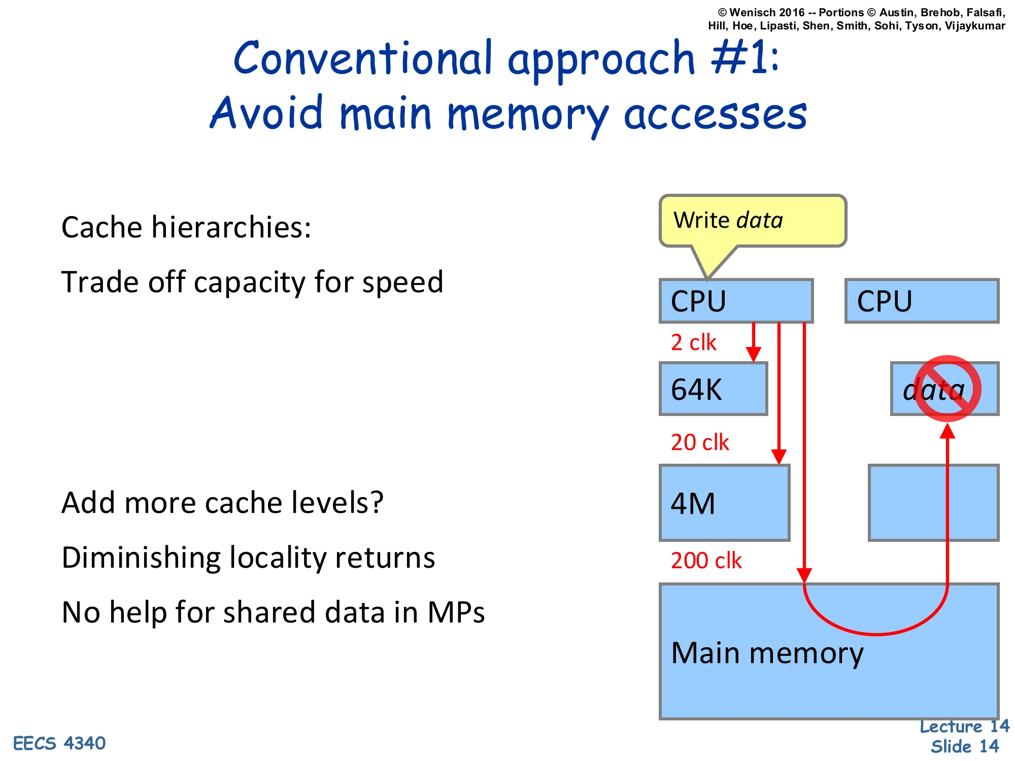
Conventional Approach #1: Avoid Main Memory Accesses
- Cache hierarchies:
- Trade off capacity for speed
- Add more cache levels?
- Diminishing locality returns
- No help for shared data in MPs
Diagram: CPU → 64K (2 clk) → 4M (20 clk) → Main memory (200 clk). Other CPU’s cache cannot be reused for data.
The first conventional response to the memory wall is to push more lines into a deeper cache hierarchy so that fewer accesses ever reach main memory. The latency numbers on the slide make the cost crystal clear: a 64 KB L1 hit is ~2 cycles, a 4 MB L2 hit is ~20 cycles, and a main-memory access is ~200 cycles. So the first miss into the L2 is already 10× the L1 hit time, and reaching DRAM is a 100× penalty. Adding a third or fourth level of cache helps less and less — the working set that fits in 4 MB but not 64 KB is much bigger than the marginal working set that would fit in 16 MB but not 4 MB, so capacity scaling shows diminishing returns once the hot working set is captured. The diagram also points out the multiprocessor wrinkle: a sibling CPU’s private cache can hold a needed line, but a deeper hierarchy on each core does nothing for these coherence-driven accesses — the data is on-chip but unreachable without a cache-to-cache transfer.
Conventional Approach #2: Hide Memory Latency
Show slide text
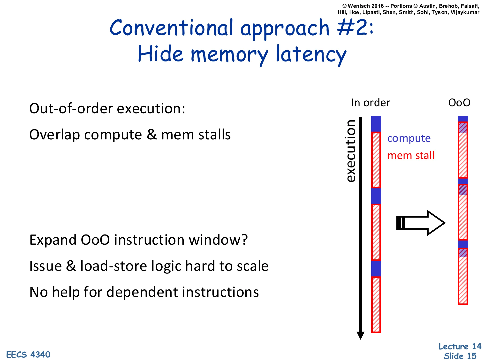
Conventional Approach #2: Hide Memory Latency
- Out-of-order execution:
- Overlap compute & mem stalls
- Expand OoO instruction window?
- Issue & load-store logic hard to scale
- No help for dependent instructions
Diagram: in-order vs. OoO timelines — OoO overlaps compute with memory stalls.
The second conventional response is out-of-order execution, which overlaps compute with memory stalls so the in-order processor’s mostly-red timeline becomes the OoO timeline with compute slipped under each red stall. The depth of overlap is bounded by the size of the OoO window — roughly the ROB capacity together with the load/store queue. There are two reasons we can’t just keep growing the window. First, scheduling logic, register-rename tables, and especially the load-store disambiguation CAMs scale super-linearly in area and power with window size; doubling capacity costs much more than 2×. Second, even an arbitrarily large window cannot hide latency for a dependent miss chain: if load B’s address depends on load A’s result, B cannot start until A returns, so a 200-cycle stall on A is followed by another 200-cycle stall on B. This second class of stalls — pointer chasing through linked structures — is exactly what the next slide highlights for server workloads, and what prefetching aims to attack.
Challenges of Server Apps
Show slide text
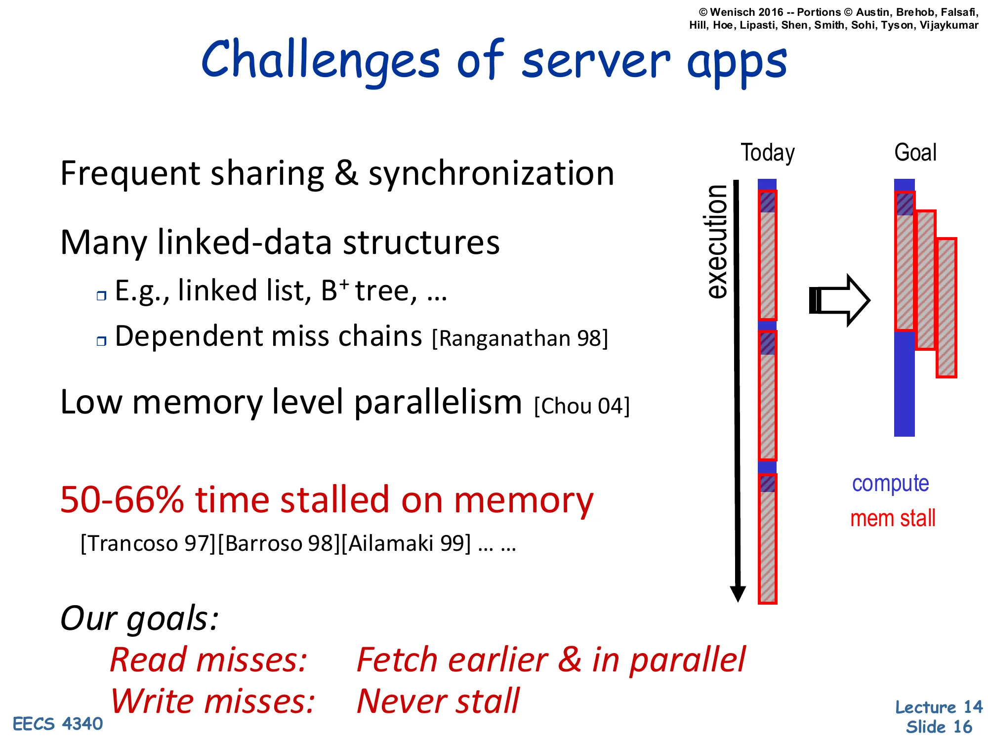
Challenges of Server Apps
- Frequent sharing & synchronization
- Many linked-data structures
- E.g., linked list, B+ tree, …
- Dependent miss chains [Ranganathan 98]
- Low memory level parallelism [Chou 04]
- 50–66% time stalled on memory [Trancoso 97][Barroso 98][Ailamaki 99] … …
Our goals:
- Read misses: Fetch earlier & in parallel
- Write misses: Never stall
Diagram: Today timeline (mostly stalled) → Goal timeline (mostly compute).
Server workloads — databases, key-value stores, web stacks — are exactly where the memory wall hurts most. Three structural reasons: shared data triggers coherence misses that no private cache helps; pointer-rich structures like linked lists and B+ trees produce dependent miss chains where one miss must complete before the next address is even known; and the resulting low memory-level parallelism leaves the OoO window mostly waiting on a single in-flight miss instead of issuing many concurrently. Empirically, multiple studies put server-app stall time at 50–66%. The lecture’s stated goal is to flip the timeline: read misses should be fetched earlier and in parallel (so the data is already in cache when demanded), and write misses should never stall the pipeline (relying on a store buffer to retire stores in the background). Prefetching is the lecture’s main answer for the read side, the rest of the slides build up the taxonomy and mechanisms.
What is Prefetching?

Show slide text
What is Prefetching?
- Fetch memory ahead of time
- Targets compulsory, capacity, & coherence misses
Big challenges:
- knowing “what” to fetch
- Fetching useless info wastes valuable resources
- “when” to fetch it
- Fetching too early clutters storage
- Fetching too late defeats the purpose of “pre”-fetching
Prefetching is the umbrella term for any mechanism — software or hardware — that issues a memory request before the processor demands the data. When the timing and address are right, what would have been a 200-cycle miss becomes a hit. Prefetching can target all three classes of cache misses: compulsory misses (first touch of a cold line), capacity misses (a working set that doesn’t fit), and even coherence misses in shared-memory multiprocessors. The two engineering challenges that frame the rest of the lecture are what and when. The what problem is accuracy: a wrong-address prefetch wastes off-chip bandwidth and may evict a useful line, hurting performance. The when problem is timeliness: a prefetch issued too early sits unused and may be evicted before demand; one issued too late doesn’t cover the miss latency. Every concrete prefetcher in the rest of the lecture is essentially a different answer to these two questions for a particular access-pattern class.
Software Prefetching
Show slide text
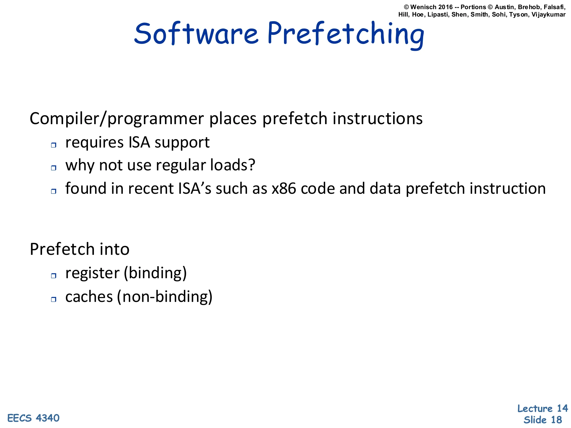
Software Prefetching
- Compiler/programmer places prefetch instructions
- requires ISA support
- why not use regular loads?
- found in recent ISA’s such as x86 code and data prefetch instruction
- Prefetch into
- register (binding)
- caches (non-binding)
Software prefetching places explicit prefetch instructions in the program — either by the compiler or the programmer — at points where a future address is computable ahead of time. A regular load could in principle fetch the line, but using a real load has two problems: it allocates a destination register, and it can fault or trigger speculation rollback if the address is bad. A dedicated prefetch instruction bypasses both issues — it has no destination register and is a no-op on faults — so it is purely a hint. Modern ISAs (x86, ARM, RISC-V) provide separate code and data prefetch instructions, sometimes with locality hints (e.g. prefetcht0/t1/t2/nta on x86 to target a specific cache level). The slide also distinguishes binding vs. non-binding prefetches: a binding prefetch reads into a register so the value is committed at fetch time (and any later write to that line is invisible to the consumer); a non-binding prefetch only warms the cache, so the demanding load sees the latest value. Most ISAs use non-binding because it is much safer in the presence of stores, coherence, and exceptions.
Software Prefetching (Cont.) — Loop Example
Show slide text
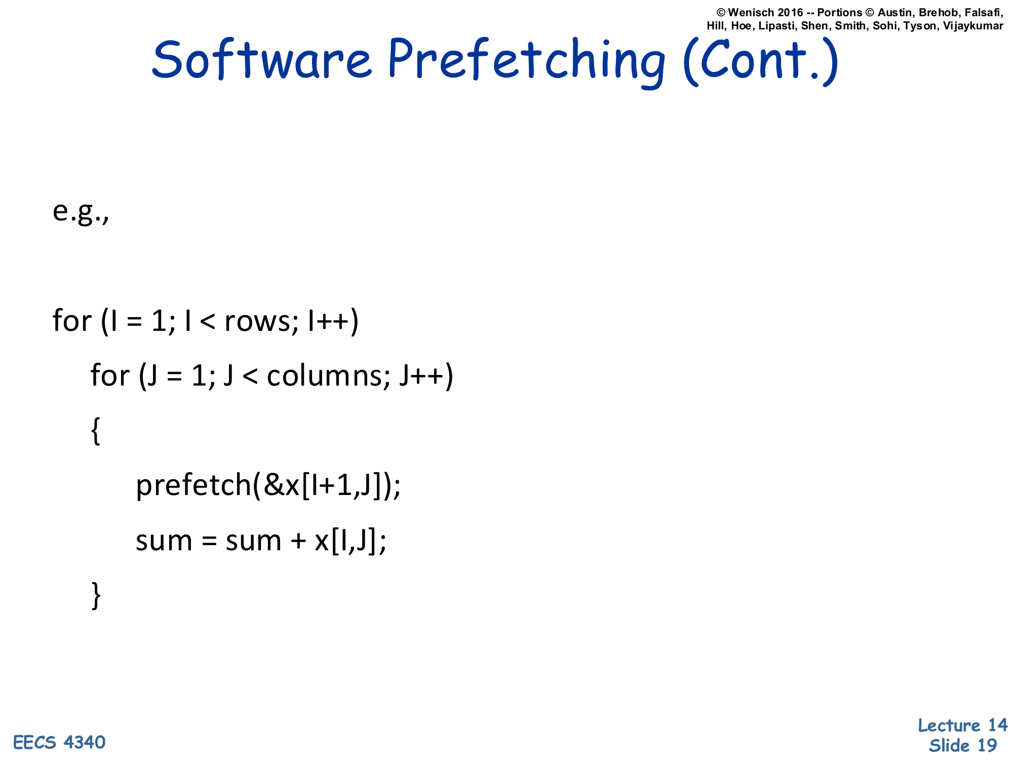
Software Prefetching (Cont.)
e.g.,
for (I = 1; I < rows; I++) for (J = 1; J < columns; J++) { prefetch(&x[I+1, J]); sum = sum + x[I, J]; }This minimal example shows why the prefetch address has to be a future address rather than the current one. The inner loop touches x[I, J] while the prefetch issues &x[I+1, J], one row ahead. The hope is that by the time the outer loop advances from row I to row I+1, the entire next row is already on its way from memory, hiding the latency. The prefetch distance — here one outer-loop iteration — is a tuning parameter: it must be large enough that the prefetched line arrives by the time it is consumed (so distance × per-iteration cycles ≥ memory latency) but not so large that the line is evicted before use. In matrix code this distance is computable at compile time given a target latency. Note also that &x[I+1, J] is touched inside the inner J loop, so each row’s lines are prefetched one cache-line at a time as the inner loop iterates — adjacent J values within the row will fall on the same line and many of those redundant prefetches are filtered by the cache (already in flight or already present).
Software Prefetching (Cont.) — DMon Examples
Show slide text
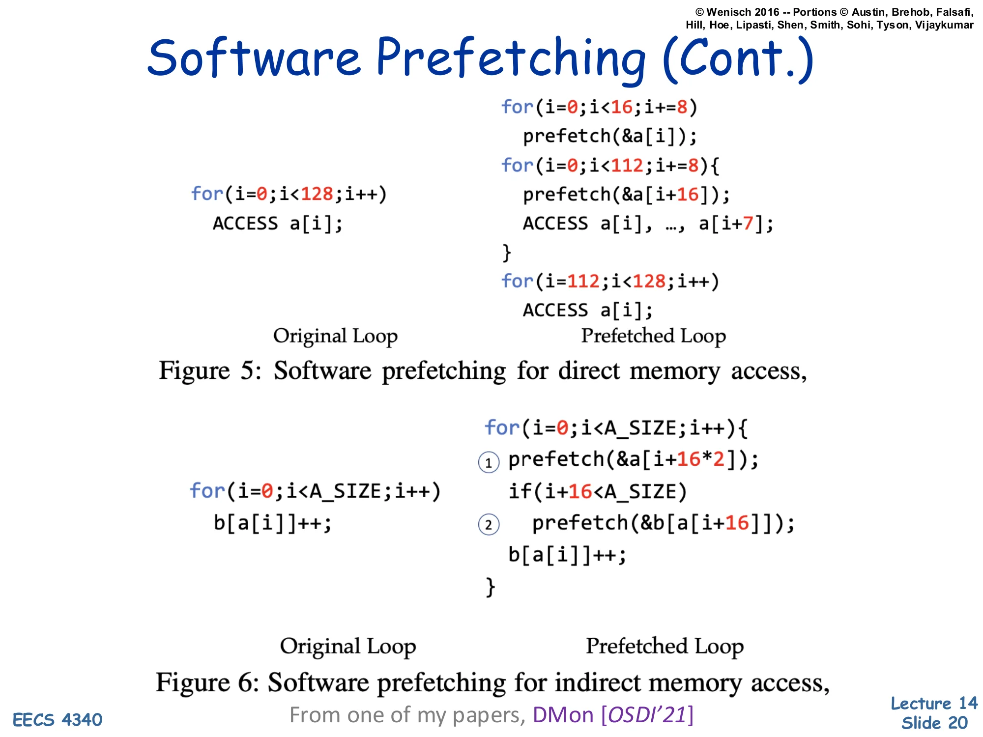
Software Prefetching (Cont.)
Figure 5: Software prefetching for direct memory access.
// Original Loopfor (i = 0; i < 128; i++)  ACCESS a[i];
// Prefetched Loop (prologue / steady-state / epilogue)for (i = 0; i < 16; i += 8)  prefetch(&a[i]);for (i = 0; i < 112; i += 8) {  prefetch(&a[i + 16]);  ACCESS a[i], …, a[i+7];}for (i = 112; i < 128; i++)  ACCESS a[i];
Figure 6: Software prefetching for indirect memory access.
// Originalfor (i = 0; i < A_SIZE; i++)  b[a[i]]++;
// Prefetchedfor (i = 0; i < A_SIZE; i++) {  // 1  prefetch(&a[i + 16*2]);  if (i + 16 < A_SIZE)    // 2    prefetch(&b[a[i + 16]]);  b[a[i]]++;}
From one of my papers, DMon [OSDI’21]
These two transformations from the DMon (OSDI’21) paper show software prefetching for the two most common access shapes. Figure 5 handles a direct sequential access — the original 128-element loop is split into three pieces: a prologue that warms up the first 16 lines (one prefetch per cache-line stride of 8 elements), a steady-state body that issues a prefetch 16 elements ahead while consuming 8 elements per iteration, and an epilogue without prefetches because all remaining lines are already in flight. Figure 6 handles indirect access b[a[i]]++ — the dereferenced address depends on a prior load, exactly the pointer-chasing chain noted earlier. To prefetch b[…] in time you must first prefetch a[i+16] (label 1) so that its value is available, and then issue a second prefetch of b[a[i+16]] (label 2). The two-stage chain is essentially a software pipeline with depth 2: prefetch-distance is 16 elements for the index array and 16 for the data array, layered. The bounds check protects the second prefetch from out-of-range access. This is exactly the kind of dependent-miss chain that hardware prefetching alone struggles with — the compiler or programmer can lay out the schedule because they know the data dependence statically.
Hardware Prefetching
Show slide text
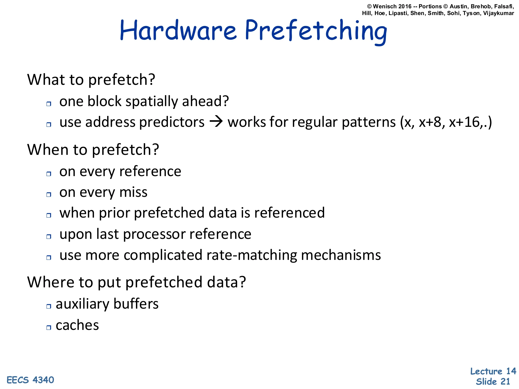
Hardware Prefetching
- What to prefetch?
- one block spatially ahead?
- use address predictors → works for regular patterns (x, x+8, x+16, …)
- When to prefetch?
- on every reference
- on every miss
- when prior prefetched data is referenced
- upon last processor reference
- use more complicated rate-matching mechanisms
- Where to put prefetched data?
- auxiliary buffers
- caches
Hardware prefetchers sit silently next to the cache and observe the demand-access stream. The slide breaks the design space along three axes. What to prefetch: the simplest answer is one block ahead (next-line prefetcher), the next is to learn an address predictor that works for regular strided patterns like x, x+8, x+16, …. When to prefetch: candidate triggers include every demand reference, every miss, the moment a previously prefetched line is first touched (which signals the prefetch was timely and another should follow), or the moment a line is evicted as a hint that it’s no longer needed. More advanced rate-matching schemes throttle prefetch issue to keep the prefetcher exactly enough lines ahead — too aggressive wastes bandwidth, too conservative defeats the purpose. Where to place prefetched data: option one is an auxiliary buffer (such as a stream buffer, slide 25) that keeps prefetches out of the demand cache and avoids polluting it; option two is to inject directly into the L1 or L2. The trade-off is pollution risk vs. coverage.
Generalized Access Pattern Prefetchers
Show slide text
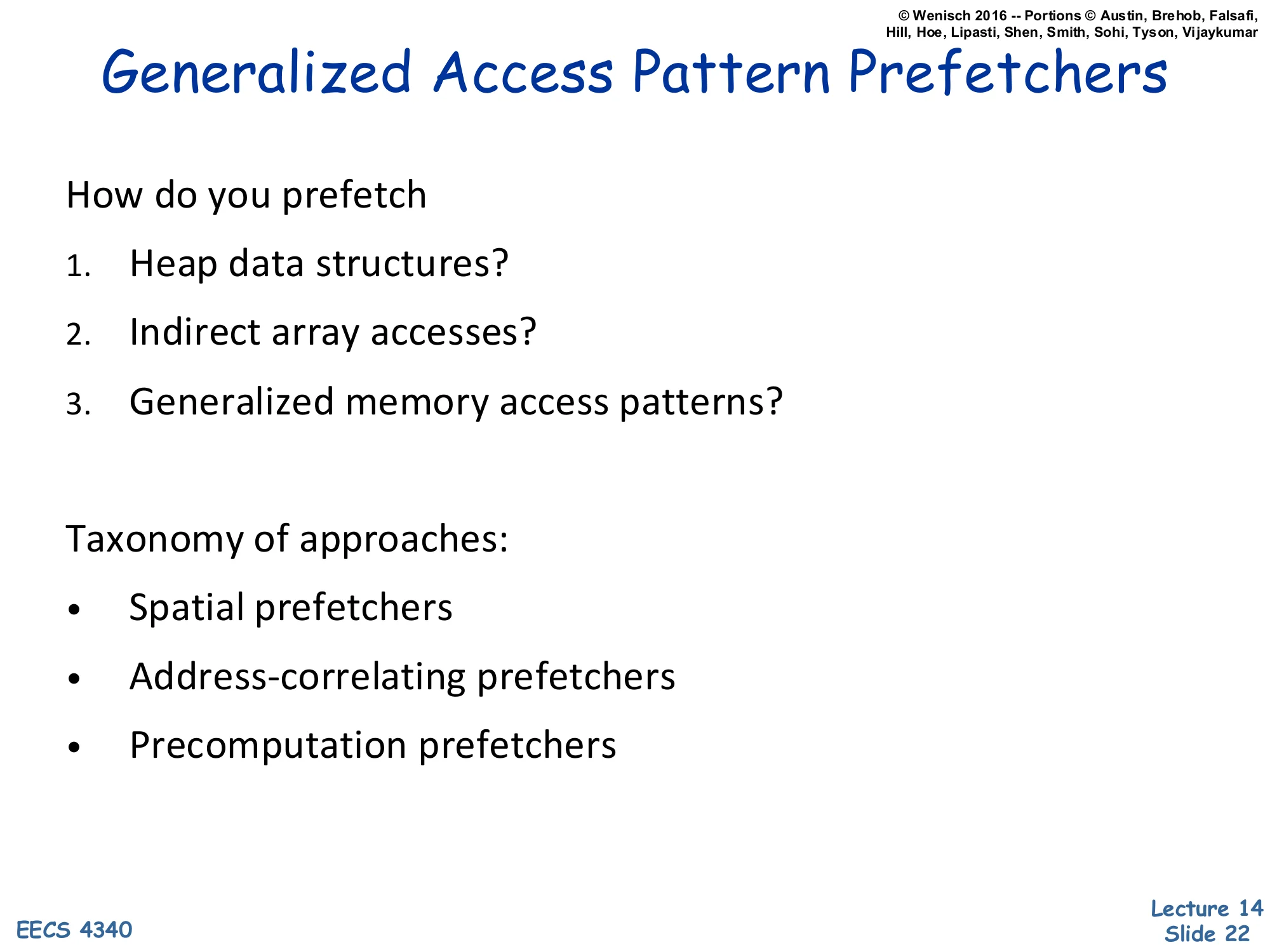
Generalized Access Pattern Prefetchers
How do you prefetch
- Heap data structures?
- Indirect array accesses?
- Generalized memory access patterns?
Taxonomy of approaches:
- Spatial prefetchers
- Address-correlating prefetchers
- Precomputation prefetchers
Real workloads stress prefetchers with three pattern classes that pure stride detection cannot capture. Heap data structures (linked lists, trees, hash chains) are pointer-chased and the next address is the value loaded by the current access. Indirect arrays like b[a[i]] require resolving an inner load before the outer address is known. Generalized patterns are anything irregular but repetitive — sparse layouts, tree traversals, database page scans — where the same relative addresses are visited each time the program revisits a structure but no simple stride exists. The lecture organizes the response into three families. Spatial prefetchers (slide 23) capture repeated layouts within a region by remembering a bitmap of touched offsets. Address-correlating prefetchers (slide 33) record “after seeing address X, address Y is likely next” — Markov-style next-address tables, or GHB delta correlations from slide 26 onward. Precomputation prefetchers (slide 41 onward) actually pre-execute the program — runahead execution speculatively runs ahead during a long miss to discover and trigger future misses. Each family handles one of the three pattern classes well.
Spatial Locality and Sequential Prefetching
Show slide text
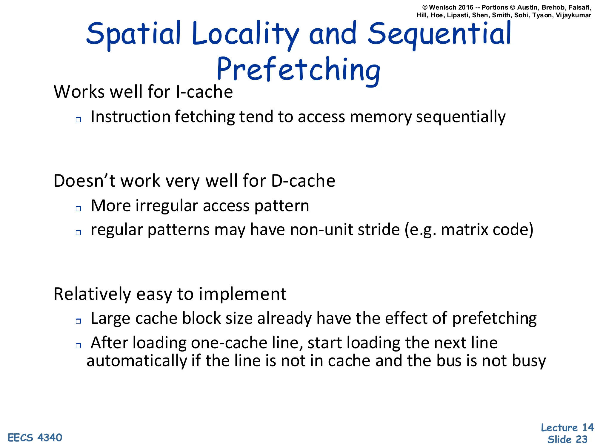
Spatial Locality and Sequential Prefetching
- Works well for I-cache
- Instruction fetching tend to access memory sequentially
- Doesn’t work very well for D-cache
- More irregular access pattern
- regular patterns may have non-unit stride (e.g. matrix code)
- Relatively easy to implement
- Large cache block size already have the effect of prefetching
- After loading one-cache line, start loading the next line automatically if the line is not in cache and the bus is not busy
Sequential next-line prefetching is the simplest hardware mechanism: on a miss for line X, also issue a prefetch for line X+1 if the bus is idle and X+1 is not already in cache. It works exceptionally well for the I-cache because instruction fetch follows the program counter and largely walks memory sequentially with the only exceptions being taken branches, which are infrequent compared to fall-through fetches. It works poorly for the D-cache because data accesses are much more irregular — pointer chases, indexed arrays, and matrix code with non-unit row strides all defeat “next line.” That said, the same principle is implicitly present everywhere: a large cache block already acts as a built-in spatial prefetcher because pulling in 64 bytes on a 4-byte access prefetches the surrounding 60 bytes for free. Slide 30 separates spatial locality (consecutive bytes are accessed close in time) from spatial correlation (the same relative offsets are accessed each time a region is revisited) — the latter is what advanced spatial prefetchers learn.
PC-based Stride Prefetchers
Show slide text
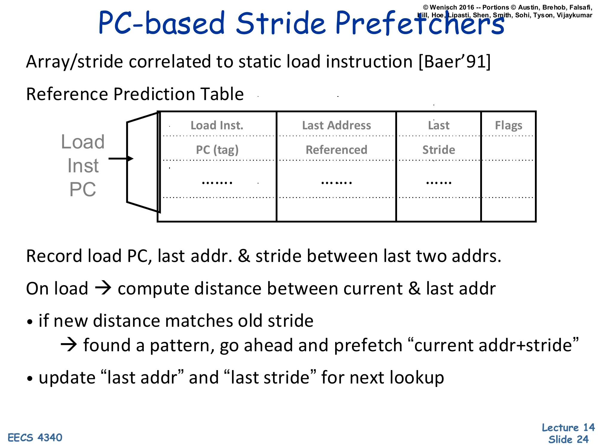
PC-based Stride Prefetchers
- Array/stride correlated to static load instruction [Baer’91]
- Reference Prediction Table
| Load Inst. PC (tag) | Last Address Referenced | Last Stride | Flags |
|---|---|---|---|
| … | … | … |
- Record load PC, last addr. & stride between last two addrs.
- On load → compute distance between current & last addr
- if new distance matches old stride
- → found a pattern, go ahead and prefetch “current addr+stride”
- update “last addr” and “last stride” for next lookup
A PC-based stride prefetcher (Baer & Chen ‘91) attaches a small table to each static load instruction. The table — the Reference Prediction Table — is indexed by the load PC and stores, per entry, the last address that instruction loaded, the last observed stride between successive accesses by that load, and confidence flags. On every executed load the prefetcher computes current_addr − last_addr and compares it to the stored stride. Match means a stable pattern is recognized: the prefetcher issues a prefetch for current_addr + stride and bumps confidence. Mismatch updates last_stride and lowers confidence; only high-confidence entries trigger prefetches. This is the right structure for matrix-style code where each static load walks an array with a fixed stride that depends on row size or struct layout — confidence filtering prevents bursts of bad prefetches when the loop transitions between phases. Compared to next-line prefetching, stride detection captures non-unit and even negative strides; compared to global address predictors it correctly handles two interleaved loads that each have their own stride because each PC has its own table entry. We will introduce this kind of per-PC stride detector as a stride prefetcher.
Stream Buffers [Jouppi]
![Stream Buffers [Jouppi] (slide 25)](/lectures/l14-prefetching/page-25.webp)
Show slide text
Stream Buffers [Jouppi]
- Each stream buffer holds one stream of sequentially prefetched cache lines
- No cache pollution
- On a load miss check the head of all stream buffers for an address match
- if hit, pop the entry from FIFO, update the cache w/ data
- if not, allocate a new stream buffer to the new miss address (may have to recycle a stream buffer following LRU policy)
- Stream buffer FIFOs are continuously topped-off with subsequent cache lines whenever there is room and the bus is not busy
- Stream buffers can incorporate stride prediction mechanisms to support non-unit-stride streams
Indirect array accesses (e.g., A[B[i]])?
Diagram: DCache and several FIFO stream buffers connected to memory interface.
Jouppi’s stream buffer is a small set of FIFOs sitting beside the L1, each tracking one detected sequential stream. On a demand miss the prefetcher checks the head of every stream buffer — if any head matches, that line is delivered to the cache and popped, opening a slot the prefetcher refills with the next sequential line; if no head matches, a stream buffer is allocated (possibly evicting an LRU stream) seeded with the miss address, and the FIFO is filled from memory in the background whenever the bus is idle. Two design choices matter. First, prefetched lines live in the buffer, not the cache, so a wrong stream cannot pollute the L1 (only when the head is consumed does the line enter the cache) — this is the stream prefetcher core idea. Second, only the FIFO head is checked, which keeps lookup cheap and forces strict in-order consumption — out-of-order access defeats the buffer. Stream buffers naturally handle multiple concurrent streams (e.g. two arrays in a loop) by giving each its own FIFO, and they can be augmented with stride detection to handle non-unit-stride streams. Indirect accesses like A[B[i]] are still a problem because the stream is not sequential at all.
Global History Buffer (GHB) [Nesbit'04]
![Global History Buffer (GHB) [Nesbit'04] (slide 26)](/lectures/l14-prefetching/page-26.webp)
Show slide text
Global History Buffer (GHB) [Nesbit’04]
- Holds miss address history in FIFO order
- Linked lists within GHB connect related addresses
- Same static load (PC/DC)
- Same global miss address (G/AC)
- Linked list walk is short compared with L2 miss latency
Diagram: Index Table indexed by Load PC → pointer into Global History Buffer; GHB entries form a chain with FIFO of miss addresses entering at the bottom.
The Global History Buffer (Nesbit & Smith ‘04) is a unifying data structure for history-based prefetchers. The GHB itself is a fixed-size FIFO of recent miss addresses — newest enter at the bottom, oldest fall off the top. A separate Index Table provides keyed entry points into the GHB; each index-table entry is a pointer to the most recent GHB slot matching that key, and GHB entries themselves link backward to earlier matches. The result is that a per-key linked list of miss-address history is materialized over the FIFO without duplicating storage. Two indexing schemes are common: PC/DC (PC-indexed delta correlation) keys by the static load PC so each load gets its own private history; G/AC (global address correlation) keys by the previous miss address itself so the predictor learns global address-to-address sequences. Nesbit’s key engineering observation is that walking the linked list is short compared with the L2 miss latency it covers, so the prefetcher has time to traverse history and issue useful prefetches before the demand miss returns. Slides 27–29 use this structure for delta correlation and slides 35–36 for global address correlation.
GHB – Deltas
Show slide text
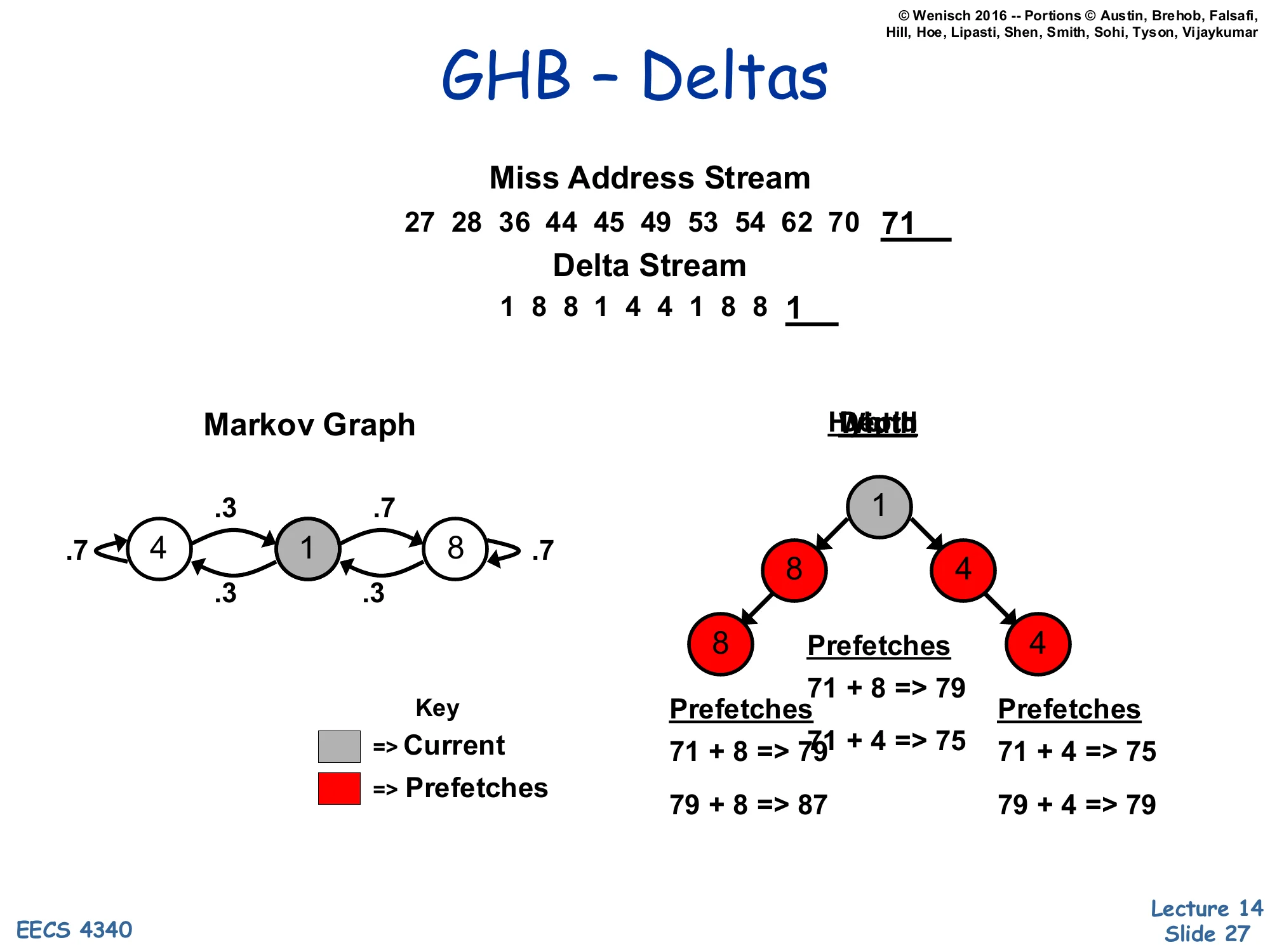
GHB – Deltas
Miss Address Stream: 27, 28, 36, 44, 45, 49, 53, 54, 62, 70, 71
Delta Stream: 1, 8, 8, 1, 4, 4, 1, 8, 8, 1
Markov Graph (cycles between deltas {1, 4, 8}):
- 4 ↔ 1: weights .3 / .7
- 1 ↔ 8: weights .7 / .3
- self-loops on 4 and 8 with weight .7
Depth tree from current delta 1: 1 → {8, 4}; 8 → 8, 4 → 4.
Prefetches (current addr 71):
- 71 + 8 → 79
- 71 + 4 → 75
- 71 + 8 → 79; 79 + 8 → 87
- 71 + 4 → 75; 79 + 4 → 79
This slide illustrates the delta version of GHB-based prefetching. Instead of correlating raw miss addresses (which have low repetition), the prefetcher correlates differences between successive misses — the delta stream. The miss stream 27, 28, 36, 44, 45, 49, 53, 54, 62, 70, 71 becomes the delta stream 1, 8, 8, 1, 4, 4, 1, 8, 8, 1. Even though the underlying addresses never repeat, the deltas cycle through a small set {1, 4, 8} and form a learnable Markov graph. Given the most recent delta is 1, the graph predicts the next delta is most likely 8 (probability .7) or 4 (probability .3), so the prefetcher issues current + 8 = 79 and current + 4 = 75 as the depth-1 candidates. Going deeper, after delta 8 the next is again either 8 or 4, so depth-2 candidates include 79 + 8 = 87 and 79 + 4 = 79 (note 75 is also reachable from a different branch). The branching factor (width) and look-ahead (depth) trade coverage against bandwidth — wider/deeper trees prefetch more aggressively but waste more bandwidth on wrong predictions. The clever part is that all this Markov structure is encoded implicitly in the GHB linked list, no explicit graph storage required.
GHB – Stride Prefetching
Show slide text
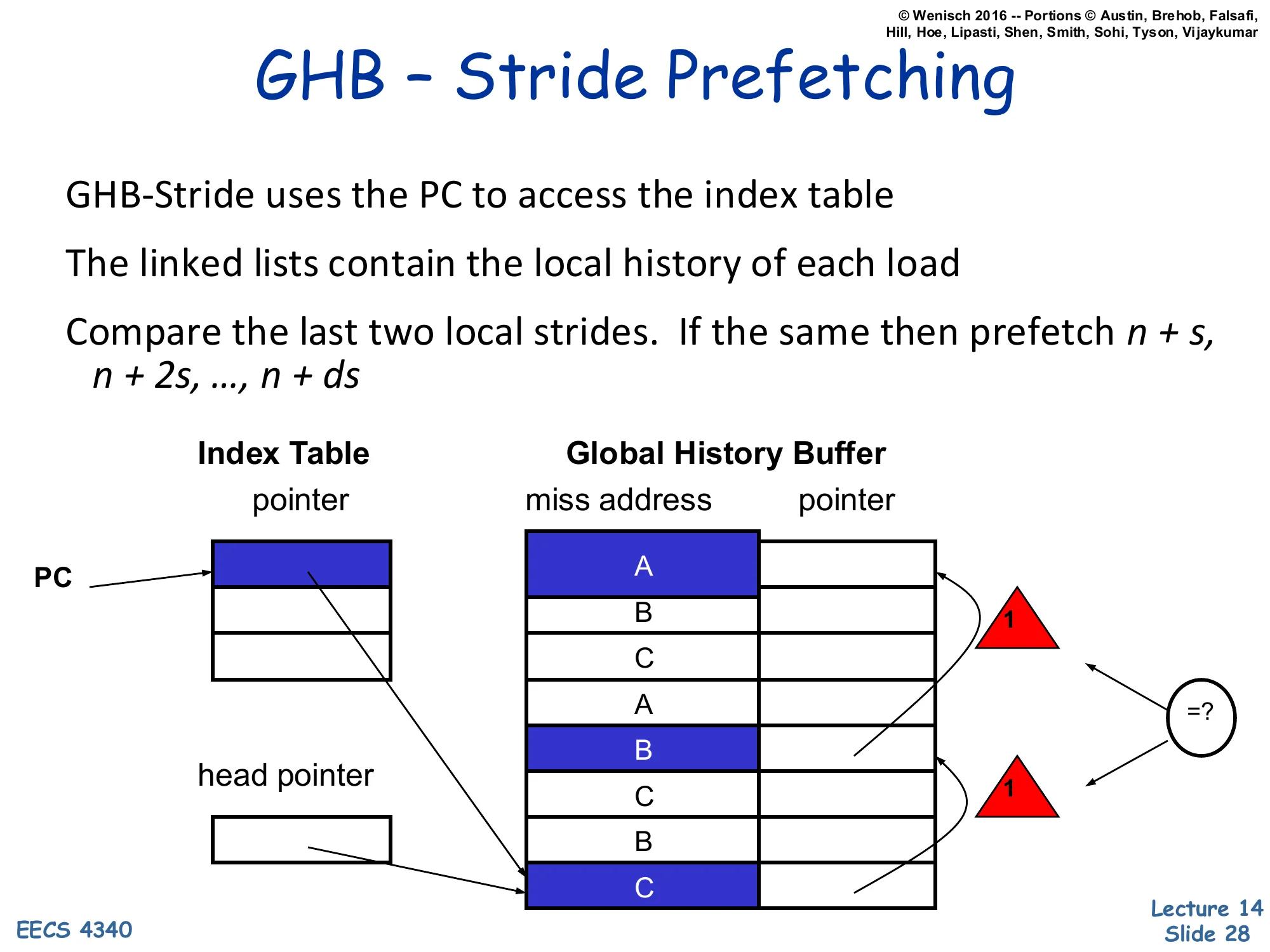
GHB – Stride Prefetching
- GHB-Stride uses the PC to access the index table
- The linked lists contain the local history of each load
- Compare the last two local strides. If the same then prefetch n + s, n + 2s, …, n + ds
Diagram: PC indexes into Index Table → pointer into Global History Buffer; the GHB miss-address column shows interleaved A, B, C, A, B, C, B, C entries; the linked list walks back to find the previous accesses by this PC. Two consecutive strides of 1 cause the equality check =? to fire and the prefetcher to issue depth-d strided prefetches.
GHB-stride re-implements the per-PC stride prefetcher from slide 24 using the GHB infrastructure. The Index Table is keyed by load PC; the GHB linked list pulls out the local history of just that PC by skipping over interleaved entries from other PCs. With three loads A, B, C interleaved in the demand stream, the linked list for PC=A walks A → A → A regardless of the interleaving. The prefetcher then computes the most recent local stride and the previous local stride and checks whether they match (the =? test in the diagram with two strides of 1). On match it issues the strided prefetch sequence n + s, n + 2s, …, n + ds for some chosen depth d, allowing it to fetch d future addresses ahead of the demand stream rather than just one. Compared with Baer & Chen ‘91, the GHB version uses a single shared address-history FIFO instead of per-PC state, so storage scales gracefully even with many active loads, and the same FIFO can be reinterpreted by other prefetcher modes (delta, global) just by changing the index key.
GHB – Delta Correlation (PC/DC)
Show slide text
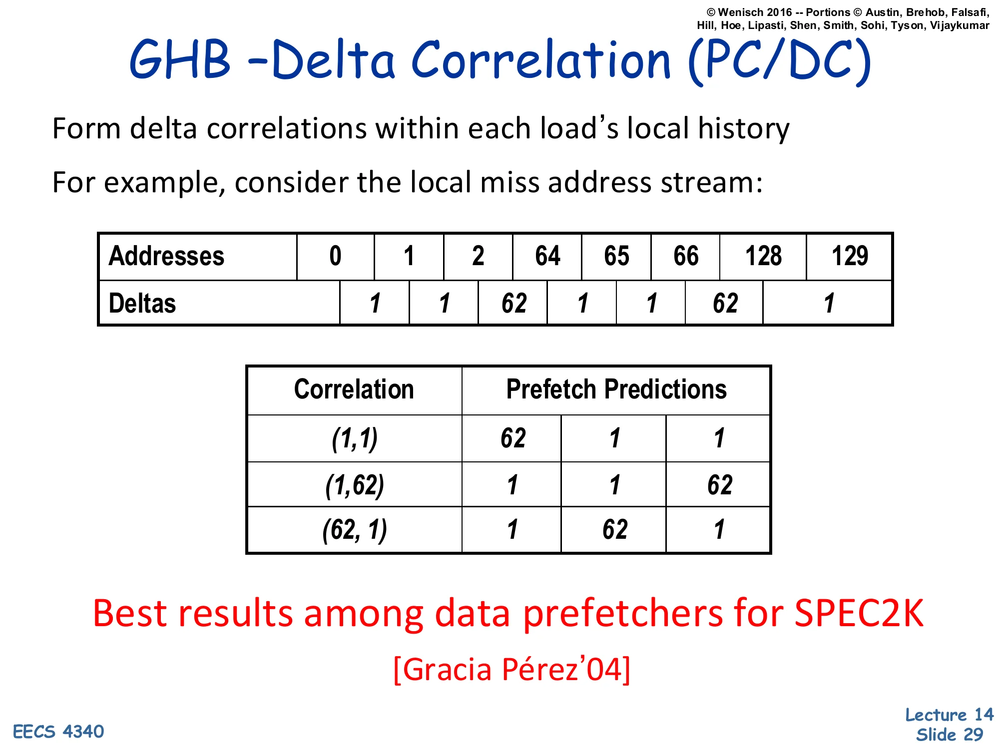
GHB – Delta Correlation (PC/DC)
- Form delta correlations within each load’s local history
- For example, consider the local miss address stream:
| Addresses | 0 | 1 | 2 | 64 | 65 | 66 | 128 | 129 |
|---|---|---|---|---|---|---|---|---|
| Deltas | 1 | 1 | 62 | 1 | 1 | 62 | 1 |
| Correlation | Prefetch Predictions |
|---|---|
| (1, 1) | 62, 1, 1 |
| (1, 62) | 1, 1, 62 |
| (62, 1) | 1, 62, 1 |
Best results among data prefetchers for SPEC2K [Gracia Pérez’04]
PC/DC (PC-indexed Delta Correlation) refines GHB stride prefetching by keying on a pair of recent deltas instead of a single stride. The example local miss stream 0, 1, 2, 64, 65, 66, 128, 129 has delta sequence 1, 1, 62, 1, 1, 62, 1 — a strict alternation that no single-delta stride detector would catch. The prefetcher forms two-delta correlations: after seeing pair (1, 1) the most recent occurrence in history was followed by deltas 62, 1, 1, so predict those three deltas; after pair (1, 62) predict 1, 1, 62; after (62, 1) predict 1, 62, 1. This Markov-of-deltas formulation captures stride patterns embedded in larger structures (here, three sequential elements per row of a 64-byte structure laid out at large offsets — typical of striding through a database page or sparse matrix). Gracia Pérez et al. (2004) reported PC/DC as the best data prefetcher across SPEC2K — an early signal that captured-pattern prefetchers, while more complex than next-line, deliver substantial real-world benefit on diverse code.
Spatial Correlation
Show slide text
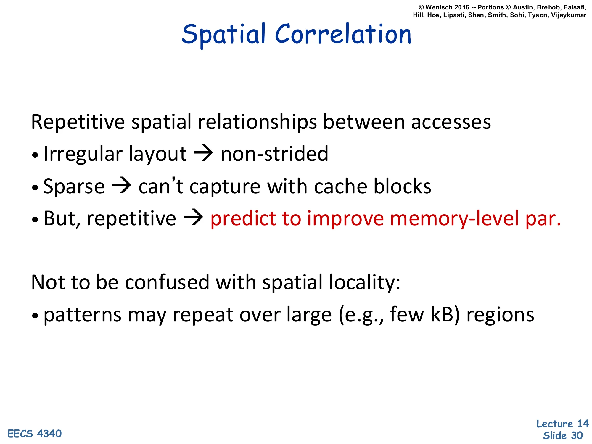
Spatial Correlation
Repetitive spatial relationships between accesses
- Irregular layout → non-strided
- Sparse → can’t capture with cache blocks
- But, repetitive → predict to improve memory-level par.
Not to be confused with spatial locality:
- patterns may repeat over large (e.g., few kB) regions
Spatial correlation is a strictly stronger property than spatial locality and motivates a whole class of spatial prefetchers. Spatial locality says “after touching byte X, byte X+δ is likely touched soon” — i.e., consecutive bytes co-occur in time, which a large cache block handles for free. Spatial correlation says “every time the program touches any byte in a region, it touches the same set of relative offsets” — the access footprint within a region is a repeatable function of the workload. Two reasons it can’t be captured by larger cache blocks. First, irregular layouts: the touched offsets within a region might be {0, 4, 64, 192} rather than a contiguous span — non-strided and not a single block. Second, sparse access: useful offsets might be spread over several kB and most of the region is dead, so loading the entire region wastes bandwidth and capacity. The repetitive-but-irregular nature is what makes spatial-correlation prefetchers profitable: by recording per-region access bitmaps and replaying them on the next region touch, they prefetch only the actually-used offsets.
Example Spatial Correlation [Somogyi'06]
![Example Spatial Correlation [Somogyi'06] (slide 31)](/lectures/l14-prefetching/page-31.webp)
Show slide text
Example Spatial Correlation [Somogyi’06]
Diagram: Database Page (8 kB) — page header in top-left, several tuple rows of mixed red/grey bytes in the middle, tuple slot index at the bottom, with arrows from the slot index up into the tuples. Right side shows the same red-byte pattern repeating over many pages of memory.
- Large-scale spatial access patterns
- Pattern is function of program
This slide grounds spatial correlation in a real workload — a database page scan. Each 8 kB page has a fixed structure: a small page header at the top, the tuple slot index at the bottom that maps slot ids to byte offsets, and tuple data rows in the middle. When the database scans a table the program reads the header, walks the slot index, and follows pointers into specific bytes of each tuple — the same relative set of red offsets is touched on every page. The right side of the diagram shows the same red-byte pattern repeating across many pages in memory. A traditional prefetcher fails here: the addresses are not strided (offsets are sparse and irregular), and the working set per page exceeds a single cache block. But spatial correlation is strong — the pattern is a property of the program, not the data — so a spatial prefetcher that records the access bitmap of one page and replays it on touching the next page can prefetch exactly the right lines without bandwidth waste. This is the workload SMS (Spatial Memory Streaming, slide 32) was designed for.
SMS Operation Summary
Show slide text
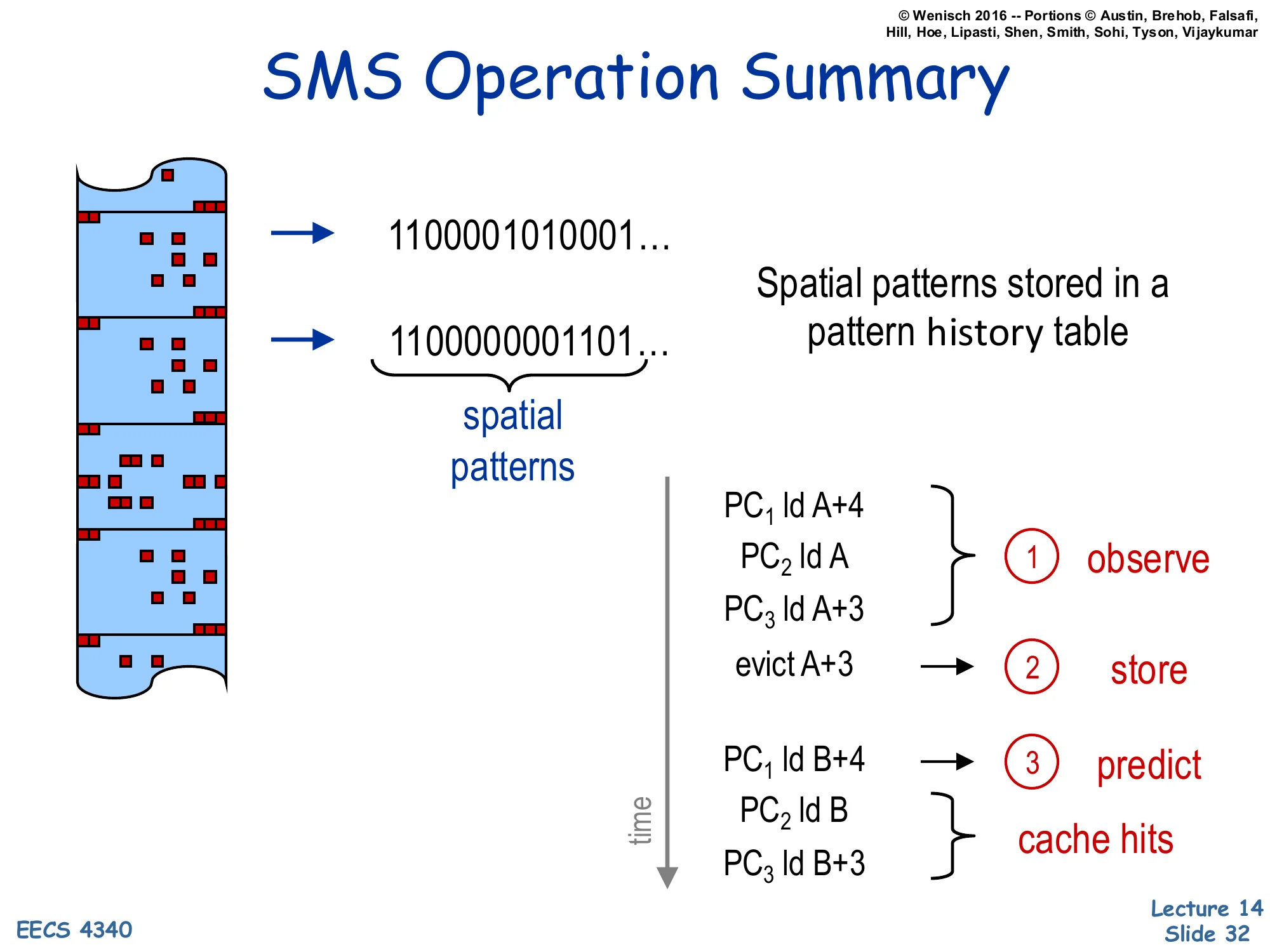
SMS Operation Summary
- Spatial patterns stored in a pattern history table (e.g., bitmap
1100001010001…,1100000001101…)
Time-ordered operation:
- observe —
PC1 ld A+4,PC2 ld A,PC3 ld A+3 - store —
evict A+3triggers writing the recorded bitmap into the pattern history table, keyed by triggering PC - predict —
PC1 ld B+4retrieves the stored pattern from the table, prefetches the matching offsets in region B;PC2 ld B,PC3 ld B+3then become cache hits
Spatial Memory Streaming (SMS) is the canonical spatial prefetcher for the database-page-style workloads on slide 31. Its operation is a three-phase cycle. Observe: while a region is alive in the cache, a per-region bitmap tracks which offsets within that region have been touched, keyed by the PC of the first access — the “triggering” load. Store: when the region is evicted (the slide shows evict A+3 as the trigger), the captured bitmap is committed to a Pattern History Table indexed by the triggering PC. Predict: when the same triggering PC later accesses a new region (PC1 ld B+4), the prefetcher looks up the stored bitmap and issues prefetches for every offset that was touched last time, applied to the new region’s base address. The follow-up demand accesses PC2 ld B and PC3 ld B+3 then hit in the cache. SMS captures repeatable spatial footprints up to several kilobytes, far beyond what a single cache block or stride prefetcher can cover, and the per-PC keying lets it distinguish different traversal patterns within the same code (header walk vs. tuple scan) cleanly.
Correlation-Based Prefetching [Charney 96]
![Correlation-Based Prefetching [Charney 96] (slide 33)](/lectures/l14-prefetching/page-33.webp)
Show slide text
Correlation-Based Prefetching [Charney 96]
Consider the following history of Load addresses emitted by a processor:
A, B, C, D, C, E, A, C, F, F, E, A, A, B, C, D, E, A, B, C, D, C
After referencing a particular address (say A or E), are some addresses more likely to be referenced next?
Markov Model (transition probabilities between states A, B, C, D, E, F):
- A → B (.6), A → C (.2), A → A (.2)
- B → C (1.0)
- C → D (.67), C → E (.2), C → F
- D → E (.33), D → C (.6)
- E → A (1.0)
- F → E (.5), F → F (.5)
Charney’s correlation-based prefetcher (1996) treats the load address stream as a discrete-time Markov process and learns the transition probabilities directly. From the example history A, B, C, D, C, E, A, C, F, F, E, A, A, B, C, D, E, A, B, C, D, C you can count, for example, that A is followed by B six out of ten times so P(B | A) = .6. The Markov model summarizes the stream as transition probabilities P(next | current) for every observed address, so after referencing A the next addresses (in expected-likelihood order) are B, C, A; after referencing E it is always A. This generalizes stride and delta prefetchers — they implicitly assume the next miss is at a fixed offset, while a Markov model can capture arbitrary irregular patterns including pointer chases, as long as they repeat. The cost is that the model needs to store transitions for every observed address, which gets large. The next slide shows the practical hardware approximation: a small Correlation Table keyed by load address, holding only the top-N most-likely successors with confidence counters.
Correlation-Based Prefetching
Show slide text
Correlation-Based Prefetching
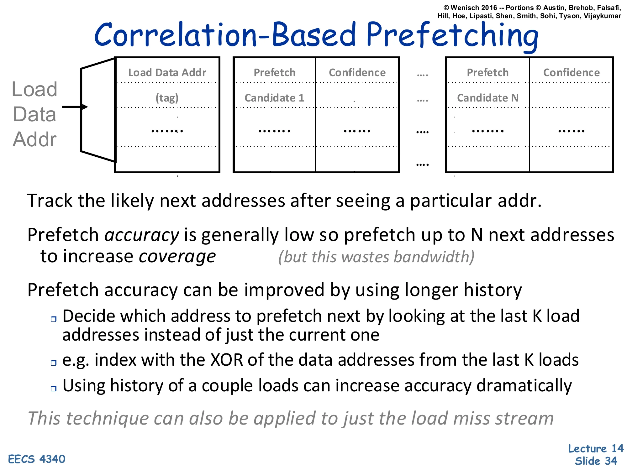
Load Data Addr → Correlation Table:
| Load Data Addr (tag) | Prefetch Candidate 1 | Confidence | … | Prefetch Candidate N | Confidence |
|---|
- Track the likely next addresses after seeing a particular addr.
- Prefetch accuracy is generally low so prefetch up to N next addresses to increase coverage (but this wastes bandwidth)
- Prefetch accuracy can be improved by using longer history
- Decide which address to prefetch next by looking at the last K load addresses instead of just the current one
- e.g., index by the XOR of the data addresses from the last K loads
- Using history of a couple loads can increase accuracy dramatically
- This technique can also be applied to just the load miss stream
The hardware realization of the Markov model is a Correlation Table indexed by the current load data address. Each entry stores up to N candidate next-addresses with confidence counters. When the current load matches an entry, the prefetcher issues prefetches for the top-N candidates simultaneously — sacrificing accuracy for coverage on the assumption that one of N is likely correct. Accuracy is improved by widening the index from “last 1” to “last K” load addresses; the slide suggests XORing the last K addresses to form a compact index, which captures multi-step context without exploding the table. Two practical wrinkles. First, indexing by every load is expensive and noisy — many load streams alias each other; restricting the table to the miss stream alone reduces noise and table pressure dramatically while still covering the long-latency events you care about. Second, the bandwidth cost of issuing N prefetches per trigger is real, so this style of correlation prefetching is most useful on workloads where the off-chip bandwidth is underutilized but AMAT is dominated by miss penalty rather than throughput.
Revisit: Global History Buffer (GHB) [Nesbit'04]
![Revisit: Global History Buffer (GHB) [Nesbit'04] (slide 35)](/lectures/l14-prefetching/page-35.webp)
Show slide text
Revisit: Global History Buffer (GHB) [Nesbit’04]
- Holds miss address history in FIFO order
- Linked lists within GHB connect related addresses
- PC/DC (de-emphasized)
- Same global miss address (G/AC)
- Linked list walk is short compared with L2 miss latency
Diagram: Index Table indexed by Miss Address → pointer into Global History Buffer; GHB FIFO of miss addresses with linked-list backpointers.
This slide returns to the Global History Buffer and emphasizes the global address-correlation mode (G/AC) instead of the per-PC mode. In G/AC, the Index Table is keyed by the miss address itself rather than by load PC. The linked list now connects all previous occurrences of that exact miss address, so the GHB chain materializes the question “what address sequences have followed this address before?” — exactly the Markov-correlation model from slides 33-34, but using the GHB FIFO as the underlying storage. The structure has the same elegance as the PC-indexed mode: storage is shared across all addresses (no fixed per-key budget), the linked-list walk is bounded by the GHB capacity, and the same prefetcher hardware can be reconfigured between PC/DC and G/AC modes by changing only the index function. This is the structural foundation for the next slide’s worked example.
GHB (G/AC) – Example
Show slide text
GHB (G/AC) – Example
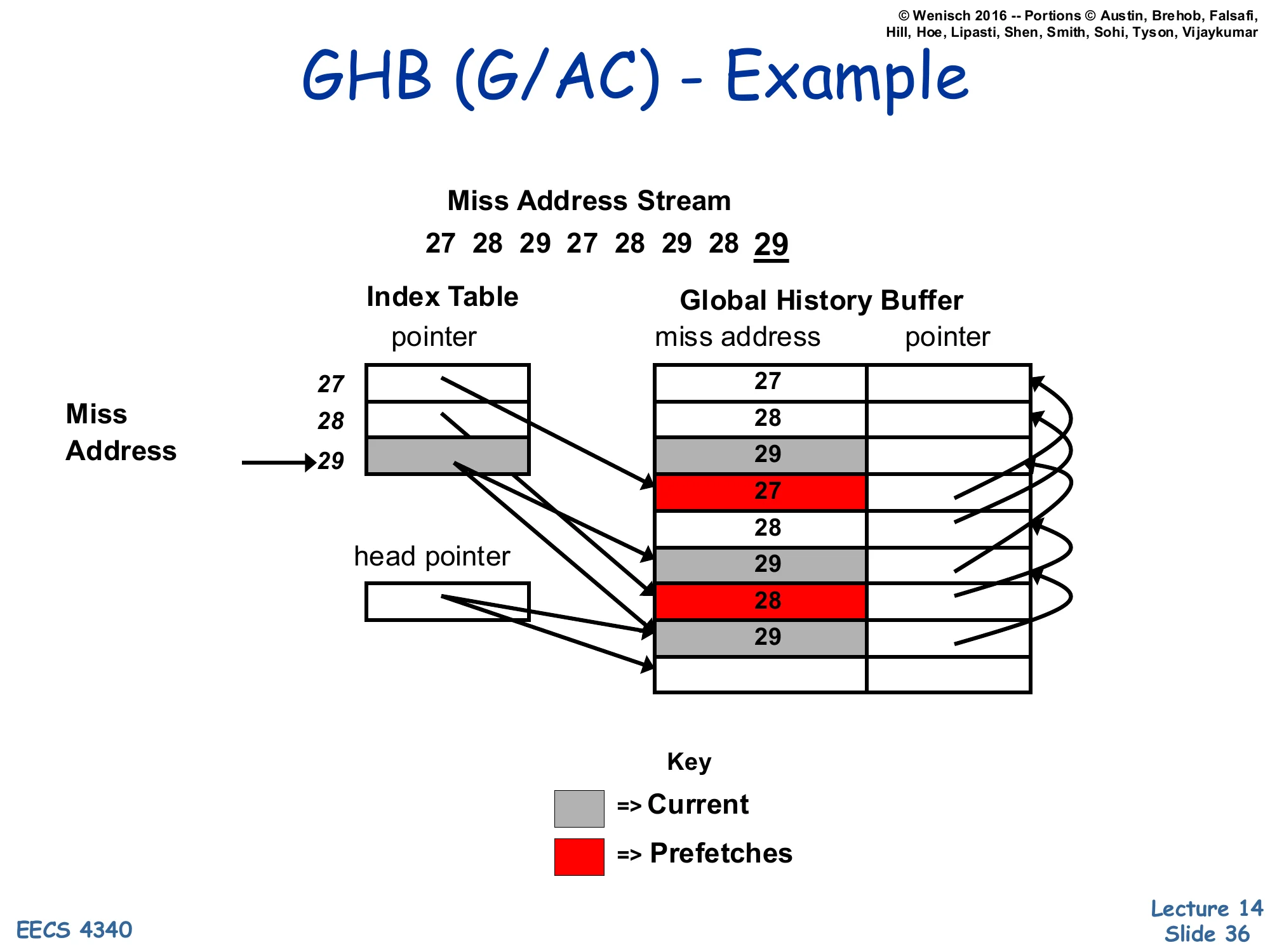
Miss Address Stream: 27, 28, 29, 27, 28, 29, 28, 29
Index Table entries point into the Global History Buffer:
| Index entry | GHB chain |
|---|---|
| 27 → … | … → 27 (older) |
| 28 → … | … → 28 → 28 → 28 |
| 29 → … (current) | 29 (current) → 29 → 29 |
Prefetches (red entries 27 and 28 in the GHB) are inserted into the cache as predictions for what follows the current 29.
This worked example shows how G/AC mode predicts. The miss stream 27, 28, 29, 27, 28, 29, 28, 29 is recorded in the GHB FIFO; the Index Table entry for address 29 points to the most recent occurrence of 29 in the GHB, which then links backward to all earlier occurrences. When the current miss is 29, the prefetcher walks the linked list of past 29s and looks at what address followed each one historically — the diagram highlights 27 and 28 in red, indicating they followed 29 in prior history (the second occurrence of 29 was followed by 27, the first by 28). The prefetcher therefore issues prefetches for both 27 and 28 as candidates for the next miss after 29. Note that this is exactly the Markov correlation model from slide 34, just stored implicitly in the GHB linked list instead of an explicit Correlation Table — same predictions, more storage-efficient, and easily reconfigurable between key modes.
Linked-Data Prefetchers
Show slide text
Linked-Data Prefetchers
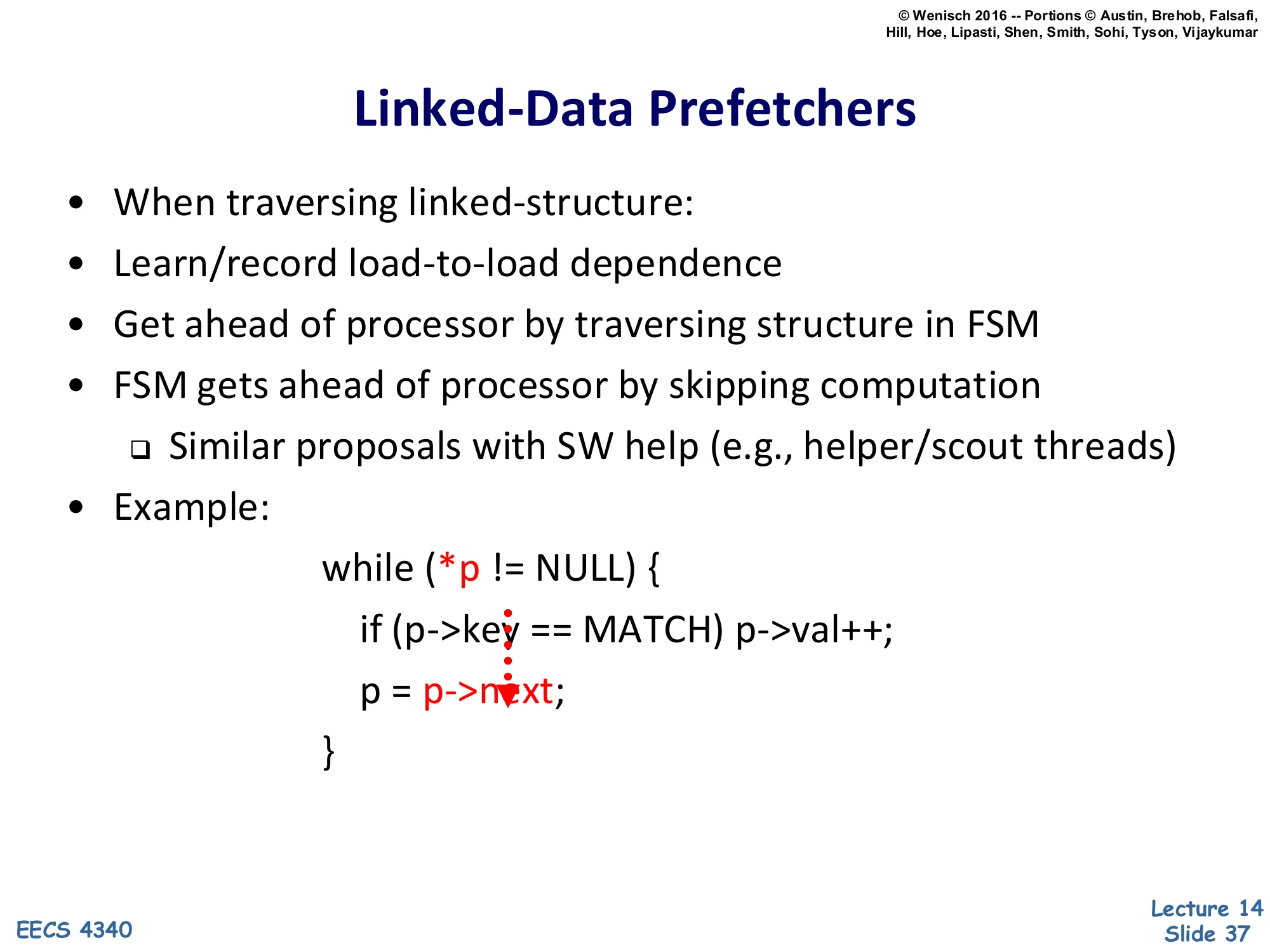
- When traversing linked-structure:
- Learn/record load-to-load dependence
- Get ahead of processor by traversing structure in FSM
- FSM gets ahead of processor by skipping computation
- Similar proposals with SW help (e.g., helper/scout threads)
- Example:
while (*p != NULL) { if (p->key == MATCH) p->val++; p = p->next;}The pointer dereferences *p, p->key, and p->next are highlighted as the core load-to-load dependence.
Spatial, stride, and address-correlation prefetchers all assume the next address is some function of previous addresses. Linked-data structures break that assumption — the next address p->next is the value loaded by the current access, so address-only history cannot predict it. The linked-data prefetcher takes a different angle: it learns load-to-load dependences in the program (which load’s value feeds which other load’s address) and uses an FSM to walk the structure ahead of the processor by skipping the intervening compute (if (p->key == MATCH) p->val++; in the example). The FSM essentially executes only the address arithmetic of the loop body — load p->next, follow it, repeat — racing ahead of the main pipeline. Software-only variants of the same idea use helper threads or scout threads that run a stripped-down version of the loop on a spare hardware context, generating prefetches via real loads. Both variants share the principle: when address dependences are too data-dependent for pattern-based prediction, just run the address-generating code itself, decoupled from the main computation.
Linked Data Structure Access
Show slide text
Linked Data Structure Access
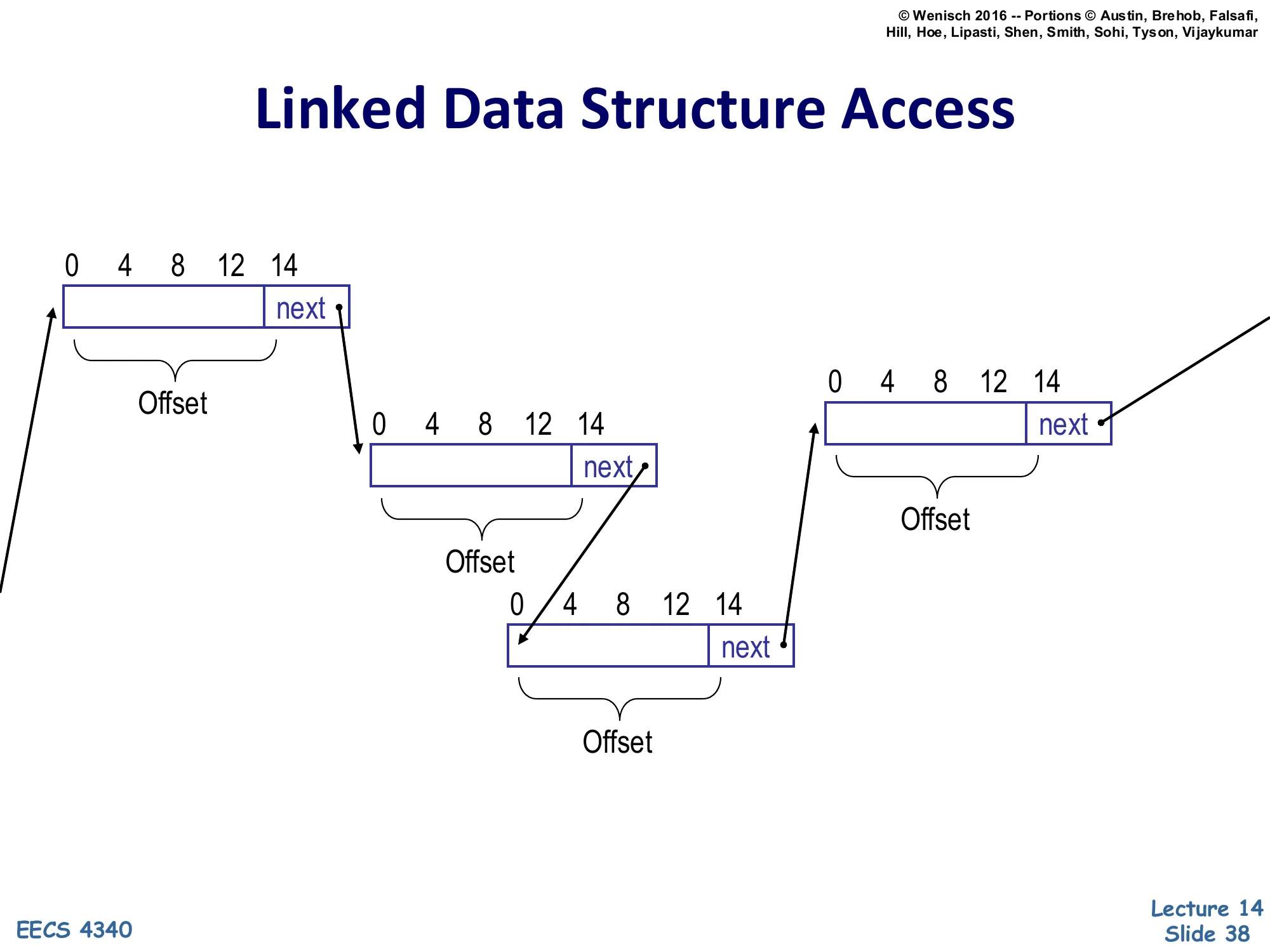
Three linked-list nodes laid out in memory, each 16 bytes wide with fields at offsets 0, 4, 8, 12, and a next pointer at offset 14. Arrows show the chain: node 1’s next points into node 2, node 2’s next points into node 3, and node 3’s next points further ahead.
Each node has the same Offset structure (data fields at the lower offsets, next pointer at offset 14).
This slide visualizes the data dependence the linked-data prefetcher must capture. Each list node is a record of the same shape — fields at byte offsets 0, 4, 8, 12, and a next pointer at offset 14 (so node size is 16 bytes plus the pointer width). The chain is built by node-to-node pointers: a load at offset 14 of node 1 returns the base address of node 2, then a load at offset 14 of node 2 returns the base address of node 3, and so on. The key structural regularity that makes hardware prefetching possible is that the offset used for the chain pointer is the same on every node (here always 14). If the prefetcher can learn the recursive template — “a load with offset 14 produces an address that becomes the base for the next load with offset 14” — it can launch the chain of dependent loads ahead of the processor. The next two slides show how to detect this template (slide 39) and how a hardware structure (slide 40, Roth et al.) actually does it.
Detecting Recursive Accesses
Show slide text
Detecting Recursive Accesses
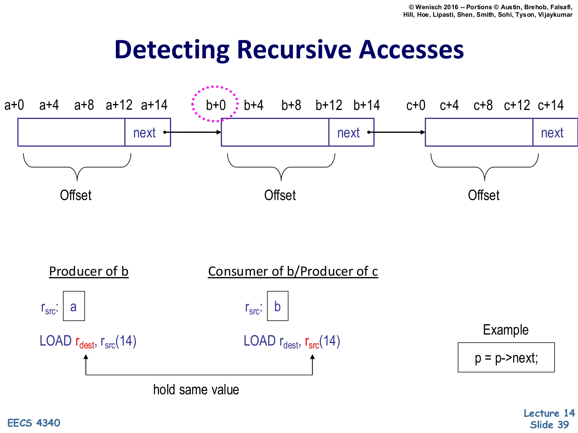
Three nodes at base addresses a, b, c; each node has fields at offsets +0, +4, +8, +12 and a next field at +14.
Producer of b: r_src: a, instruction LOAD r_dest, r_src(14)
Consumer of b / Producer of c: r_src: b, instruction LOAD r_dest, r_src(14)
hold same value — the two r_src registers in successive list iterations hold the same dynamic value link.
Example: p = p->next;
Detecting a recursive access boils down to recognizing a pattern of two related loads in the dynamic trace. The producer load at base address a issues LOAD r_dest, r_src(14) with r_src holding a; it returns the value b (the next pointer). The consumer load at base address b issues the same instruction template LOAD r_dest, r_src(14) but with r_src holding b. The crucial observation is that the value loaded by the producer (b) is the base register used by the consumer — the producer’s destination and the consumer’s source register hold the same value at different points in time. If the prefetcher hardware can detect this value flow between two loads with the same offset (14 here), it has identified a recursive chain of arbitrary length. The classic source-level pattern that produces this trace is p = p->next; inside a loop; the FSM that walks the chain just performs the same offset-14 load over and over, using the previous load’s result as the next base, racing arbitrarily far ahead of the demand stream.
Roth, Moshovos, Sohi (HW) [Roth'98]
![Roth, Moshovos, Sohi (HW) [Roth'98] (slide 40)](/lectures/l14-prefetching/page-40.webp)
Show slide text
Roth, Moshovos, Sohi (HW) [Roth’98]
Producer of b (r_src: a): PC-A: LOAD r_dest, r_src(14)
Consumer of b / Producer of c (r_src: b): PC-B: LOAD r_dest, r_src(14)
hold same value
Potential Producer Window:
| Memory Value Loaded | Producer Instruction Address |
|---|---|
| b | PC-A |
Correlation Table:
| Producer Inst. Address | Consumer Inst. Address | Consumer Inst. Template |
|---|---|---|
| PC-A | PC-B | LOAD r, r(14) |
Roth, Moshovos, and Sohi (1998) propose a hardware linked-data prefetcher that materializes the producer-consumer relationship of slide 39 in two tables. The Potential Producer Window is a small recent-loads buffer: each completed load deposits the loaded value (e.g., b) and the loading instruction’s PC (PC-A). When a new load executes and its base register holds a value that matches an entry in the window — i.e., it consumes a value some recent load produced — the prefetcher records (producer PC, consumer PC, consumer instruction template) in the Correlation Table. Once an entry is in the table, every later execution of PC-A that produces a value v immediately fires the consumer template LOAD r, r(14) against v as a prefetch — effectively running the next iteration’s address arithmetic ahead of the main pipeline. The same correlation can be chained: the prefetched consumer becomes a new producer, so the FSM walks the linked list as far ahead as latency budget allows. Notice the entries are PCs and templates, not addresses — the table is data-independent and works for any traversal of any linked structure in the program.
Runahead Execution [Mutlu'03]
![Runahead Execution [Mutlu'03] (slide 41)](/lectures/l14-prefetching/page-41.webp)
Show slide text
Runahead Execution [Mutlu’03]
Memory-level parallelism of large window without building it!
When oldest instruction is L2 miss:
- Checkpoint state and enter runahead mode
In runahead mode:
- Instructions speculatively pre-executed
- To discover other L2 misses
- Processor continues to run
Runahead mode ends when the original L2 miss returns:
- Checkpoint is restored and normal execution resumes
Runahead execution (Mutlu et al. 2003) is a precomputation prefetcher that piggybacks on the existing OoO core to expose memory-level parallelism without enlarging the ROB. The trigger is a long-latency miss that reaches the oldest ROB entry — at that point the pipeline would normally stall for the full memory latency. Instead the core checkpoints architectural state and enters runahead mode: it keeps executing speculatively past the missing load, treating the missing load’s destination register as invalid (INV) and propagating the INV taint through dependent instructions. Useful work happens for the independent instructions: they execute normally and any loads they perform issue real memory requests. Those requests hit, miss, and warm the caches for free. When the original miss finally returns the core discards the runahead speculative state, restores the checkpoint, and resumes from the original missing load — but now any L2 misses that were discovered during runahead are already in flight (or in cache), so the dependent miss chain is parallelized after the fact. The net effect is the memory-level parallelism of a much larger window without paying the area or critical-path cost of actually building one.
Runahead Example
Show slide text
Runahead Example
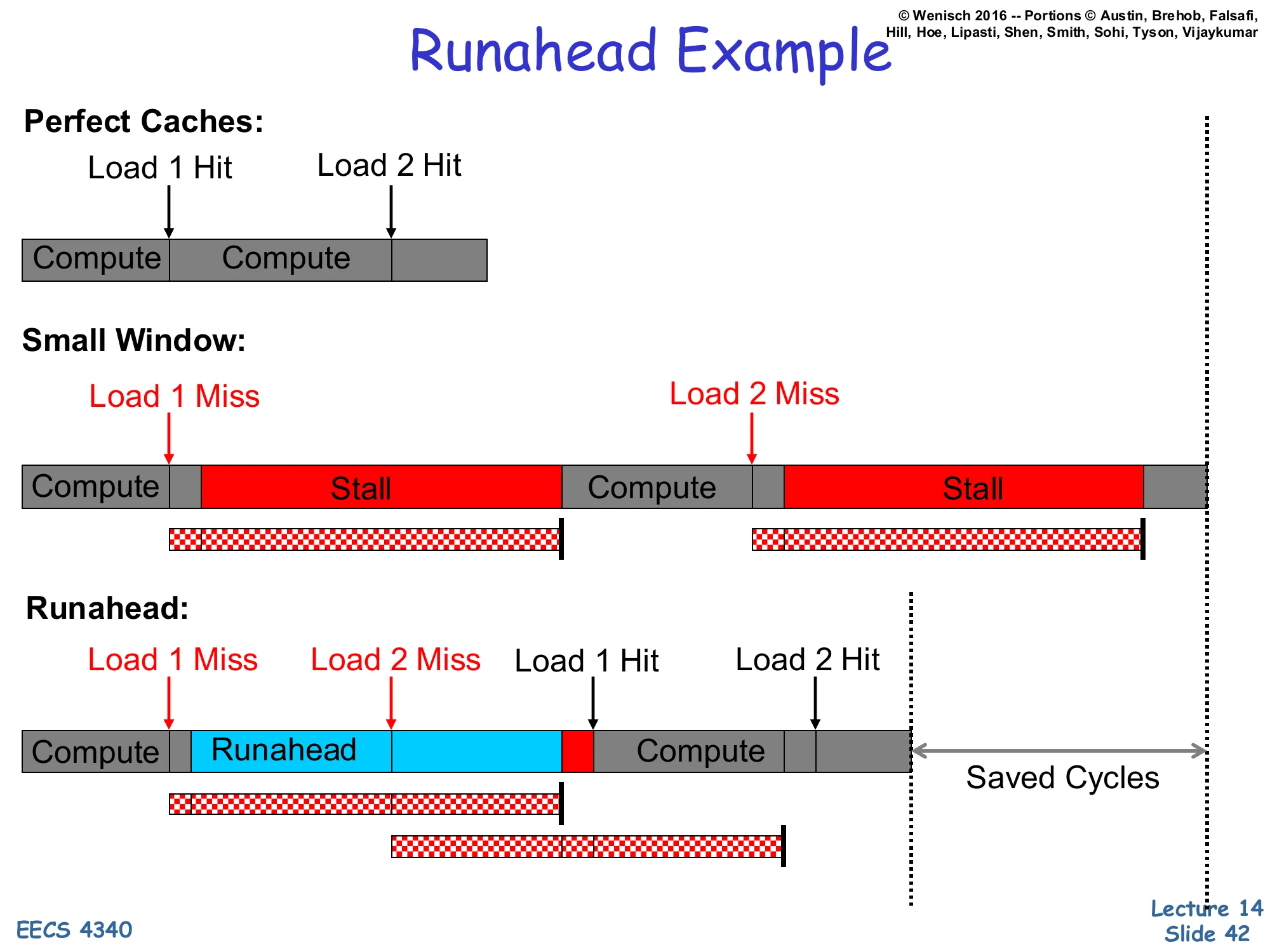
Perfect Caches: Compute → (Load 1 Hit) → Compute → (Load 2 Hit) — short timeline.
Small Window: Compute → Load 1 Miss → Stall → Compute → Load 2 Miss → Stall — two serial stalls separated by compute.
Runahead: Compute → Load 1 Miss → Runahead (during which Load 2 Miss is discovered) → Compute → Load 1 Hit → Load 2 Hit. The Load 1 and Load 2 miss latencies overlap, yielding Saved Cycles.
This timeline diagram makes the value of runahead concrete. With perfect caches both loads hit and the program is just two compute phases plus two trivial accesses. With a small window and two L2 misses (Load 1, Load 2) the pipeline stalls for the full miss latency on each, serially: Load 2 cannot even issue until Load 1’s stall is over because the stall blocks the ROB. Runahead breaks the serialization. As soon as Load 1 misses and reaches the head of the ROB, the core enters runahead and continues executing speculatively. During this window Load 2 is encountered and issued as a real memory request — its miss latency now overlaps with the remainder of Load 1’s miss latency. When Load 1 returns, the core leaves runahead, restores its checkpoint, and re-executes from Load 1; Load 1 hits (cached during runahead’s resolution) and Load 2 also hits because its line arrived during the overlap. The Saved Cycles on the right of the timeline equal roughly the latency of one full miss — exactly the memory-level parallelism a much larger OoO window would have provided, but achieved with a bounded amount of checkpoint state and existing pipeline hardware.
Benefits of Runahead Execution
Show slide text
Benefits of Runahead Execution
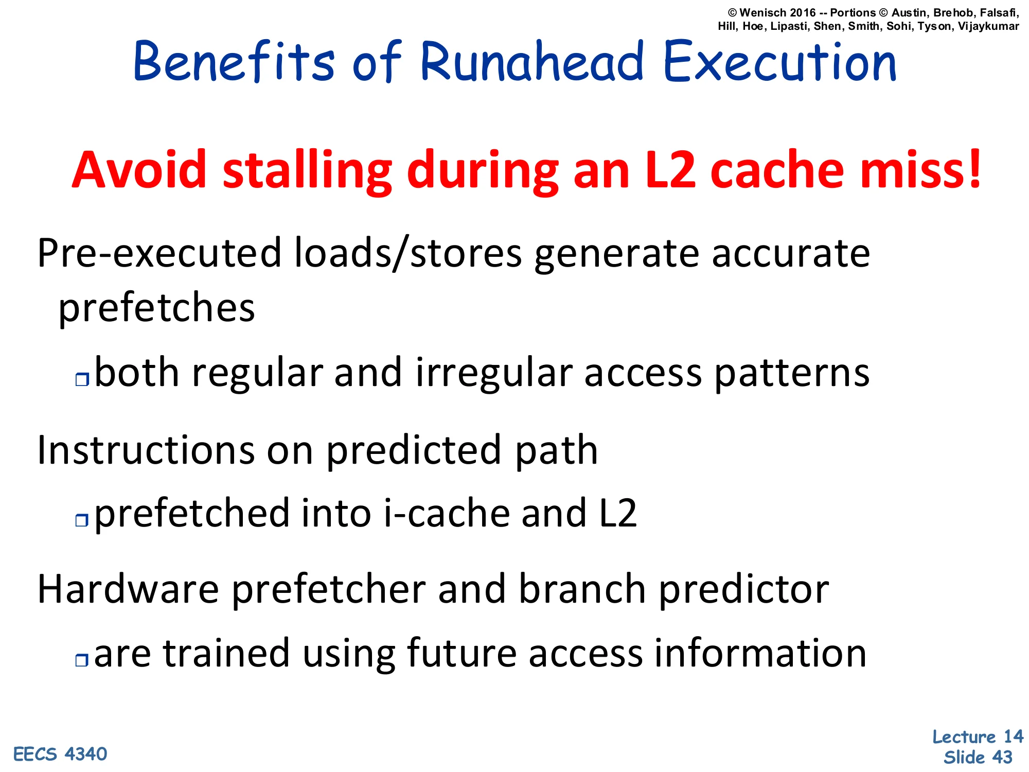
Avoid stalling during an L2 cache miss!
- Pre-executed loads/stores generate accurate prefetches
- both regular and irregular access patterns
- Instructions on predicted path
- prefetched into i-cache and L2
- Hardware prefetcher and branch predictor
- are trained using future access information
The benefits of runahead generalize beyond just data prefetching. First, because runahead actually executes the instruction stream (rather than predicting addresses statistically), the prefetches it generates are exactly the addresses the program will demand once it resumes — accurate for both regular and irregular patterns, including pointer chasing where stride and correlation prefetchers fail. Second, runahead also fetches and decodes ahead, so instructions on the predicted control-flow path get prefetched into the i-cache and L2 — runahead is therefore an instruction prefetcher in addition to a data prefetcher. Third, every runahead instruction trains the existing hardware structures: the branch predictor sees real branch outcomes (well, runahead-mode outcomes) and updates accordingly, and the regular hardware prefetcher sees future miss addresses and tunes its tables. The compounded effect is that runahead converts an idle full-miss stall into useful speculative work that benefits virtually every speculation engine in the pipeline.
Improving Cache Performance: Summary
Show slide text
Improving Cache Performance: Summary
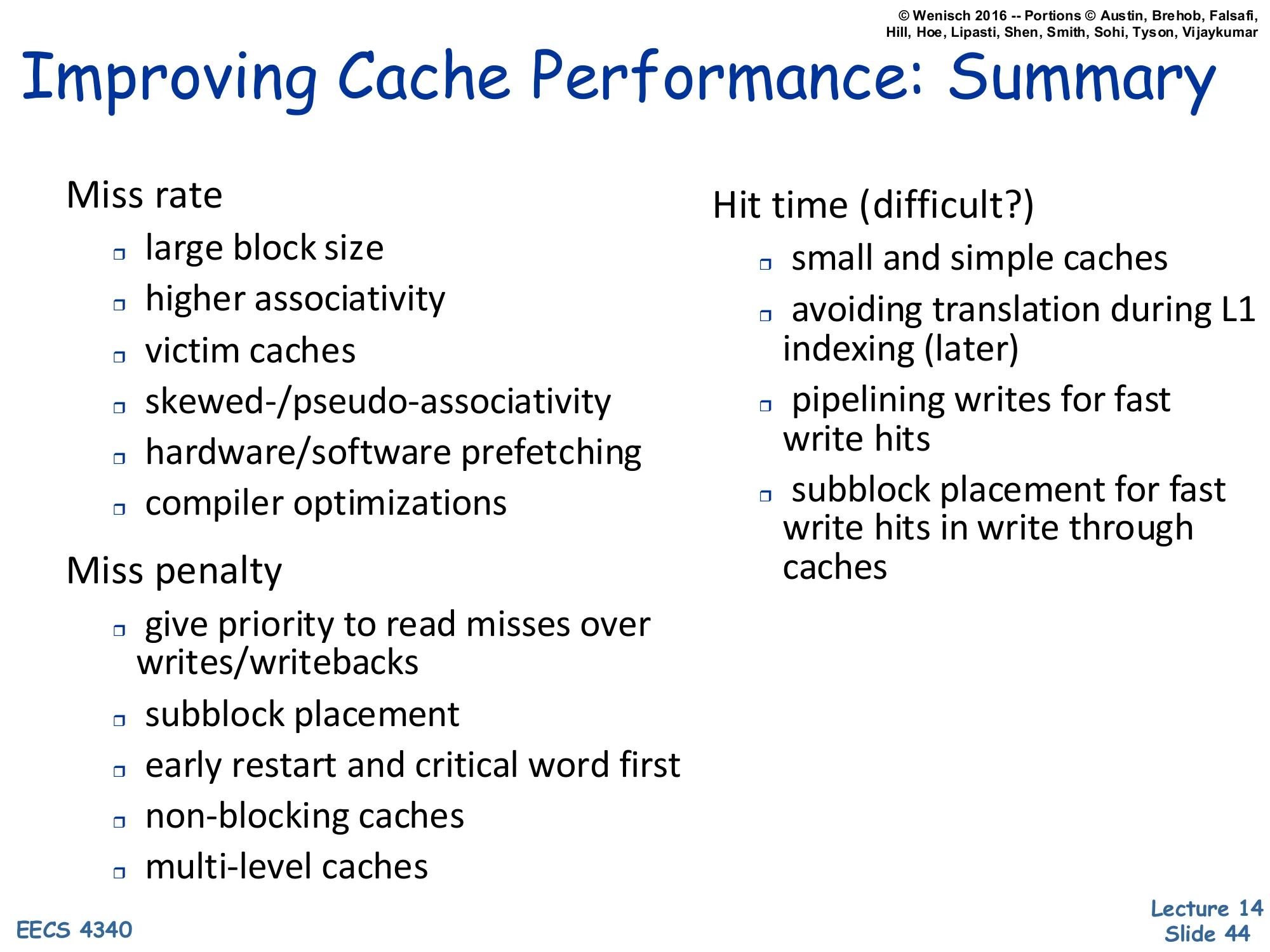
Miss rate
- large block size
- higher associativity
- victim caches
- skewed-/pseudo-associativity
- hardware/software prefetching
- compiler optimizations
Miss penalty
- give priority to read misses over writes/writebacks
- subblock placement
- early restart and critical word first
- non-blocking caches
- multi-level caches
Hit time (difficult?)
- small and simple caches
- avoiding translation during L1 indexing (later)
- pipelining writes for fast write hits
- subblock placement for fast write hits in write through caches
This wrap-up slide organizes everything from the cache lectures by which term of AMAT = hit time + miss rate × miss penalty each technique attacks. The miss-rate column lists architectural and software techniques that reduce how often we miss: larger blocks cut compulsory misses, higher associativity cuts conflict misses, victim caches and skewed associativity address residual conflicts, and hardware/software prefetching (the topic of this lecture) cuts compulsory and capacity misses by anticipating accesses. The miss-penalty column is what reduces the cost of each miss: read priority to avoid being held up by writes, subblock placement to load less data, early restart and critical-word-first to forward the wanted word ASAP, non-blocking caches to overlap multiple in-flight misses, and multi-level caches to amortize the worst-case penalty. The hit-time column is the hardest to improve because it sits on the critical path: keep the L1 small and simple, avoid TLB translation in the indexing path (covered in the next lecture on virtual memory), and use pipelined writes and subblock placement to keep write hits cheap. Every concrete technique you’ve seen this semester lives in exactly one of these three columns.
Readings
Show slide text
Readings
For today:
- A primer on hardware prefetching, https://doi.org/10.1007/978-3-031-01743-8
For next Monday:
- Appendix L, http://www.cs.yale.edu/homes/abhishek/abhishek-appendix-l.pdf
- Architectural and Operating System Support for Virtual Memory, https://doi.org/10.1007/978-3-031-01757-5
Announcements

Show slide text
Announcements
- Project #4
- Due: 1-May-26
- Final project presentation
- May 4, 2026
- 8:40 to 9:50 AM
- 8 minutes per group, schedule on Courseworks