L10 · Branch Prediction

L10 · Branch Prediction

Topic: branch-prediction · 54 pages

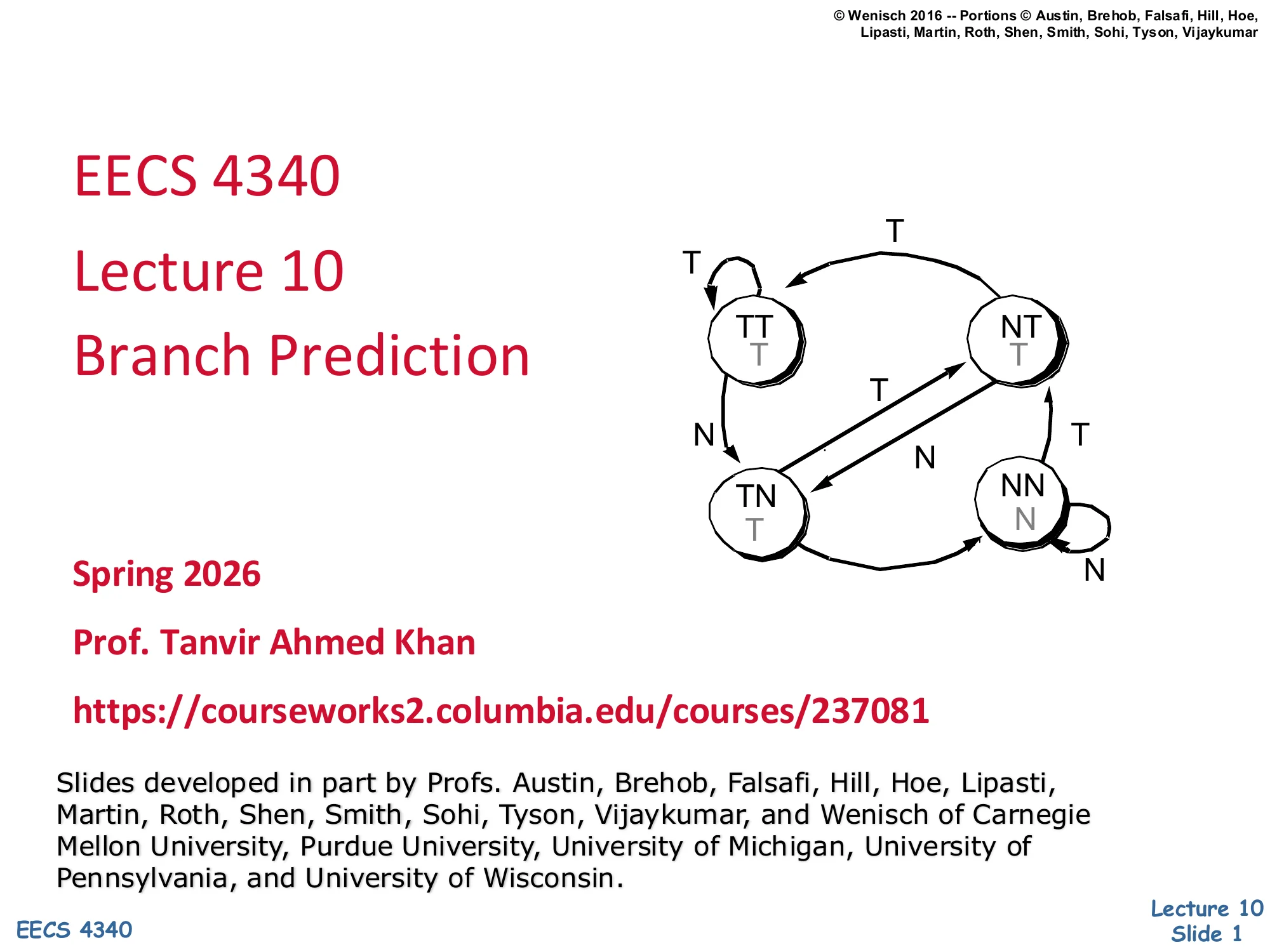
EECS 4340 Lecture 10 — Branch Prediction

Slide 1

Announcements

Slide 2

Show slide text

Announcements

Project #4

• Due: milestone 3, 8-April-26
• In-person mandatory project check-in
  • 8:40–8:50 AM: CCDYMP
  • 8:50–9:00 AM: G13
  • 9:00–9:10 AM: GaPiChiXuXu
  • 9:10–9:20 AM: OoO
  • 9:20–9:30 AM: RISCy Whisky
  • 9:30–9:40 AM: SIX
  • 9:40–9:50 AM: UNI

Optional project meetings

• Mondays and Wednesdays during my office hours

https://courseworks2.columbia.edu/courses/237081

Readings

Slide 3

Show slide text

Readings

For today:

• H & P Chapter 3.3
• A comparison of dynamic branch predictors that use two levels of branch history — https://dl.acm.org/doi/abs/10.1145/165123.165161

For next Monday:

• H & P Chapter 3.9
• McFarling: Combining Branch Predictors

Recap: Memory Scheduling

Slide 4

Out-of-Order Memory Operations

Slide 5

Show slide text

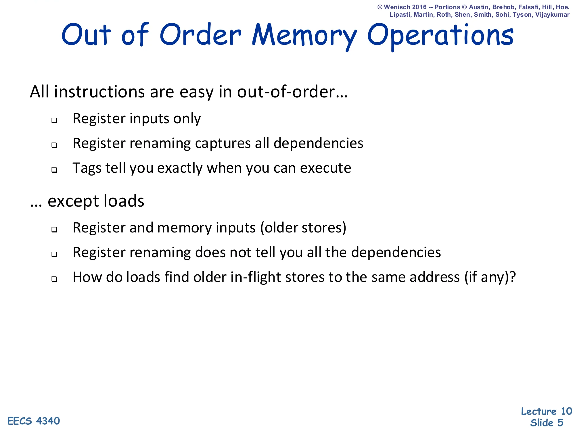
Out of Order Memory Operations

All instructions are easy in out-of-order…

• Register inputs only
• Register renaming captures all dependencies
• Tags tell you exactly when you can execute

…except loads

• Register and memory inputs (older stores)
• Register renaming does not tell you all the dependencies
• How do loads find older in-flight stores to the same address (if any)?

This slide pinpoints why loads are the awkward case for Tomasulo-style out-of-order execution. For ALU and store-data instructions, every input is a register, so register renaming captures all true dependencies and the reservation-station tag broadcast on the CDB tells the consumer exactly when its operands are ready. Loads break that clean picture: a load’s value depends not just on its address operands but also on any older in-flight store to the same memory address. Renaming cannot expose that dependence because the address is computed dynamically and the store and load may use entirely different register names. So the question — which older un-retired store, if any, holds the value this load should read? — is answered not by tags but by an associative search over the in-flight store list. That requirement is exactly what motivates the store queue and load queue structures introduced over the following slides.

Dynamic Reordering of Memory Operations

Slide 6

Show slide text

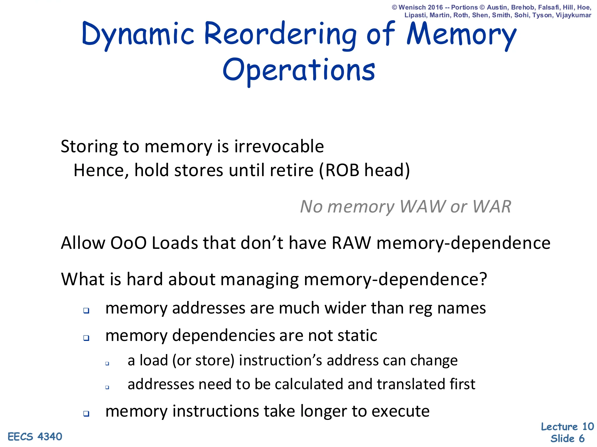
Dynamic Reordering of Memory Operations

Storing to memory is irrevocable

• Hence, hold stores until retire (ROB head)

No memory WAW or WAR

Allow OoO Loads that don’t have RAW memory-dependence

What is hard about managing memory-dependence?

• memory addresses are much wider than reg names
• memory dependencies are not static
  • a load (or store) instruction’s address can change
  • addresses need to be calculated and translated first
• memory instructions take longer to execute

Because a store to memory cannot be undone once the cache or memory is written, in-order-commit machines hold every store in a buffer until the ROB head retires it. This commit-time release of stores automatically eliminates memory WAW and memory WAR hazards — there is exactly one architectural store at any time, in program order. The remaining task is to allow loads to execute out of order whenever they have no RAW memory dependence on an older un-retired store. Memory-dependence is harder than register dependence for three reasons listed on the slide: addresses are 32–64 bits versus a handful of register-name bits (so wide CAM searches are expensive); the addresses are dynamic — recomputed each iteration and possibly translated through the TLB; and the memory pipeline is multi-cycle, so an older store may not even know its own address when a younger load is ready to issue. These three observations frame the rest of the recap.

Some Trivial Ways to Handle Loads

Slide 7

Show slide text

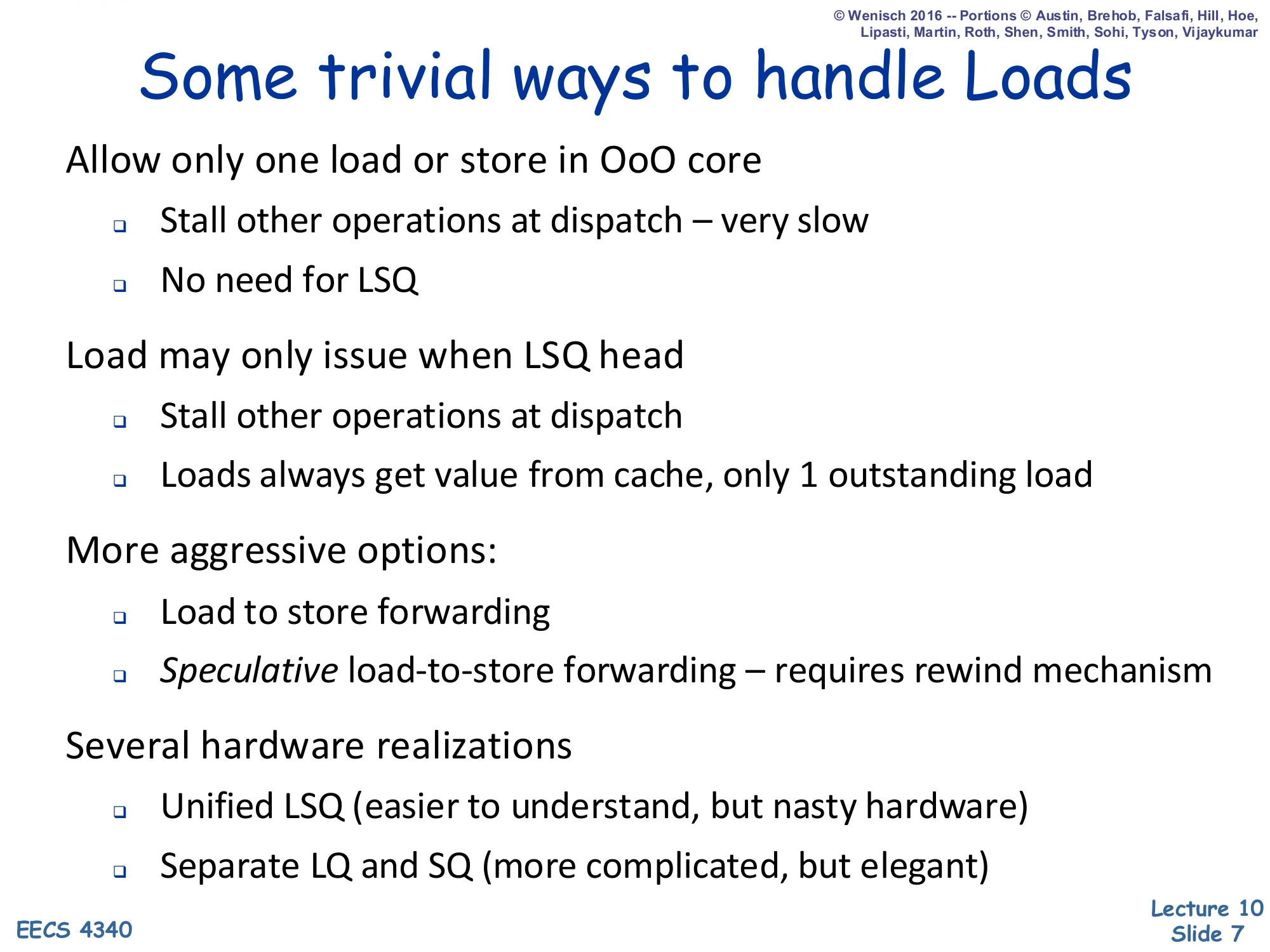
Some trivial ways to handle Loads

Allow only one load or store in OoO core

• Stall other operations at dispatch — very slow
• No need for LSQ

Load may only issue when LSQ head

• Stall other operations at dispatch
• Loads always get value from cache, only 1 outstanding load

More aggressive options:

• Load to store forwarding
• Speculative load-to-store forwarding — requires rewind mechanism

Several hardware realizations

• Unified LSQ (easier to understand, but nasty hardware)
• Separate LQ and SQ (more complicated, but elegant)

The slide walks up a ladder of correctness-versus-performance tradeoffs for memory operations. The cheapest correct design only allows one in-flight load or store, eliminating the need for any associative load/store queue but throwing away most memory-level parallelism. Slightly better, the design allows multiple memory ops in flight but only lets a load issue once it sits at the head of the LSQ — preserving program order without speculation. The aggressive options bring back parallelism: store-load forwarding lets a load read an older un-retired store from the store queue when their addresses match, and speculative forwarding lets a load issue before older store addresses are even known, at the cost of a rewind/replay mechanism if the speculation later turns out wrong. Finally, the slide previews two organizational choices used by real CPUs: a unified LSQ that holds both loads and stores in one CAM versus a split design with separate LQ and SQ structures, which is the choice the next several slides examine in detail.

HW#2: Split Queues

Slide 8

Show slide text

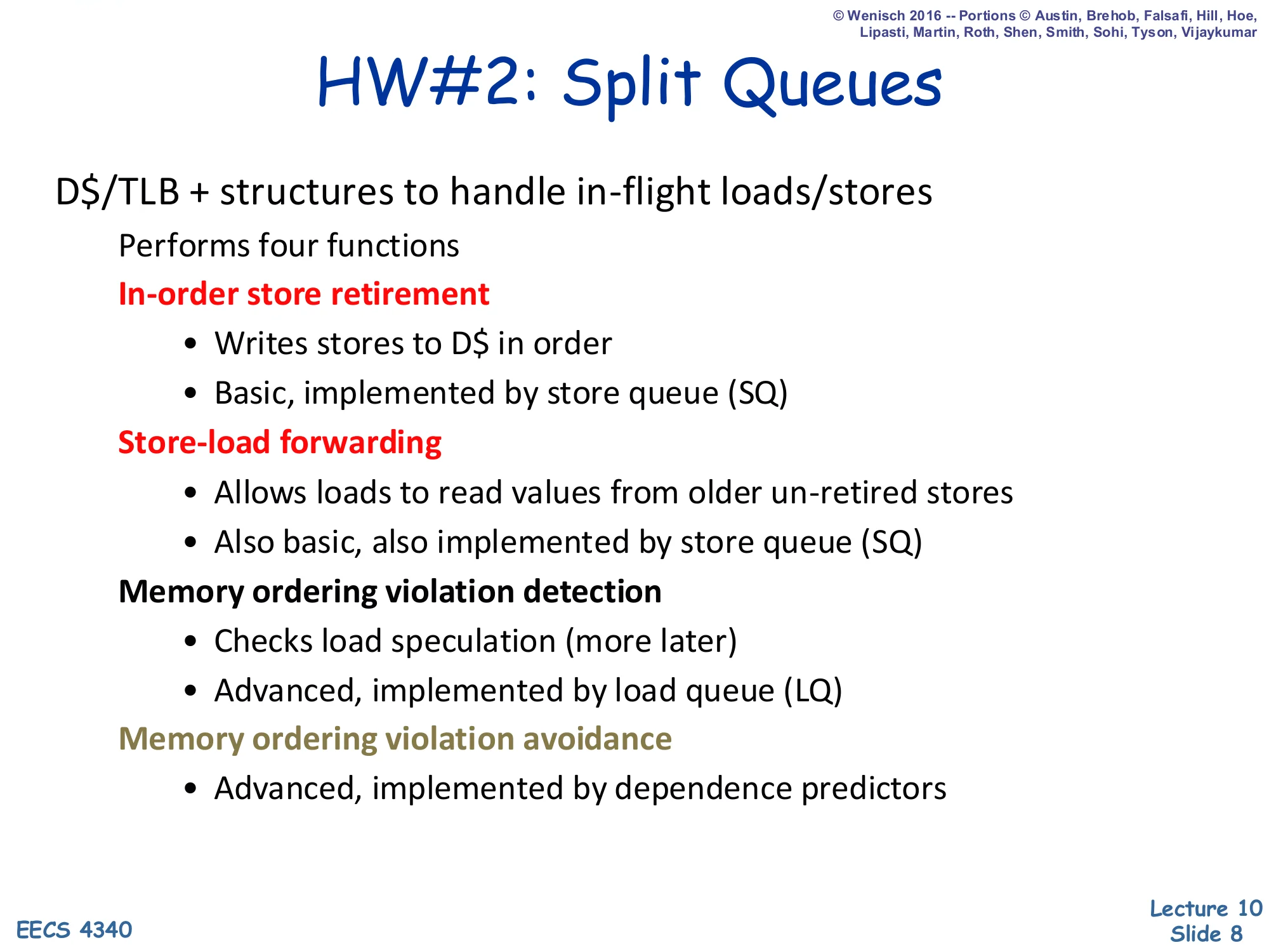
HW#2: Split Queues

D$/TLB + structures to handle in-flight loads/stores

Performs four functions

In-order store retirement

• Writes stores to D$ in order
• Basic, implemented by store queue (SQ)

Store-load forwarding

• Allows loads to read values from older un-retired stores
• Also basic, also implemented by store queue (SQ)

Memory ordering violation detection

• Checks load speculation (more later)
• Advanced, implemented by load queue (LQ)

Memory ordering violation avoidance

• Advanced, implemented by dependence predictors

This slide divides the four jobs that the load and store queues collectively perform. The two basic jobs — in-order commit of stores into the D-cache and store-to-load forwarding when a younger load matches an older un-retired store — both live in the store queue (SQ), because both depend on knowing the program-ordered set of pending writes. The two advanced jobs require the load queue (LQ): once loads are allowed to issue speculatively past older stores with unknown addresses, the LQ must detect when an older store’s address resolves to one a younger load already speculated past, which is a memory ordering violation — and trigger a flush. Avoiding those flushes proactively requires dependence predictors such as Store-Sets, which learn which load/store PCs collide and force conservative scheduling for them.

Simple Data Memory FU: D$/TLB + SQ

Slide 9

Show slide text

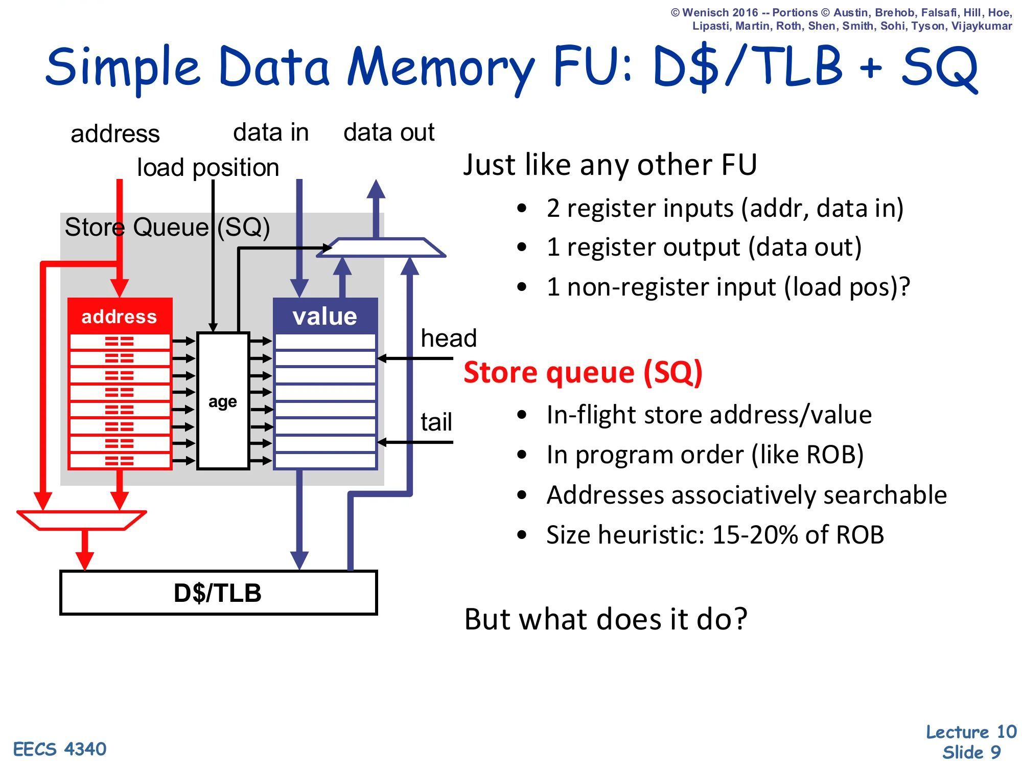
Simple Data Memory FU: D$/TLB + SQ

Just like any other FU

• 2 register inputs (addr, data in)
• 1 register output (data out)
• 1 non-register input (load pos)?

Store queue (SQ)

• In-flight store address/value
• In program order (like ROB)
• Addresses associatively searchable
• Size heuristic: 15-20% of ROB

But what does it do?

From the rest of the OoO core, the data-memory functional unit looks almost ordinary: it consumes an address register and a data register, and produces a data register on a load. The novelty is the extra non-register input, load position — a pointer that tells the unit where the load sits in program order, so it can search backward through the store queue for older stores. The SQ itself is a circular FIFO indexed in program order (mirroring the ROB), with associatively searchable address fields. The 15–20% of ROB sizing heuristic is the standard rule of thumb: with roughly one store every five or so dynamic instructions, an SQ much smaller than that becomes the OoO bottleneck, while one much larger is wasted CAM area. The closing question — what does it do? — is answered concretely on the next slides: in-order retire and store-load forwarding.

D$/TLB + SQ + LQ

Slide 10

Show slide text

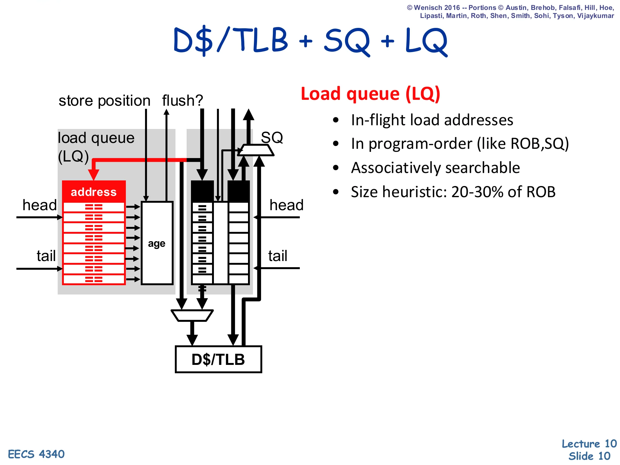
D$/TLB + SQ + LQ

Load queue (LQ)

• In-flight load addresses
• In program-order (like ROB, SQ)
• Associatively searchable
• Size heuristic: 20-30% of ROB

Adding the load queue alongside the store queue turns the data-memory unit into a two-CAM structure: every store searches the LQ to detect already-issued speculative loads to its (newly known) address, and every load searches the SQ to forward from older pending stores. The LQ also has a flush output that signals a memory ordering violation: when an older store discovers it shares an address with a younger load that already issued and read stale data from the cache, the violating load and everything dispatched after it must be squashed and re-fetched. Because there are typically more loads than stores in flight, the LQ is sized 20–30% of ROB versus the SQ’s 15–20%. Both queues share the underlying D-cache and TLB datapath through arbitration logic at the bottom of the diagram.

R10K Data Structures

Slide 11

Show slide text

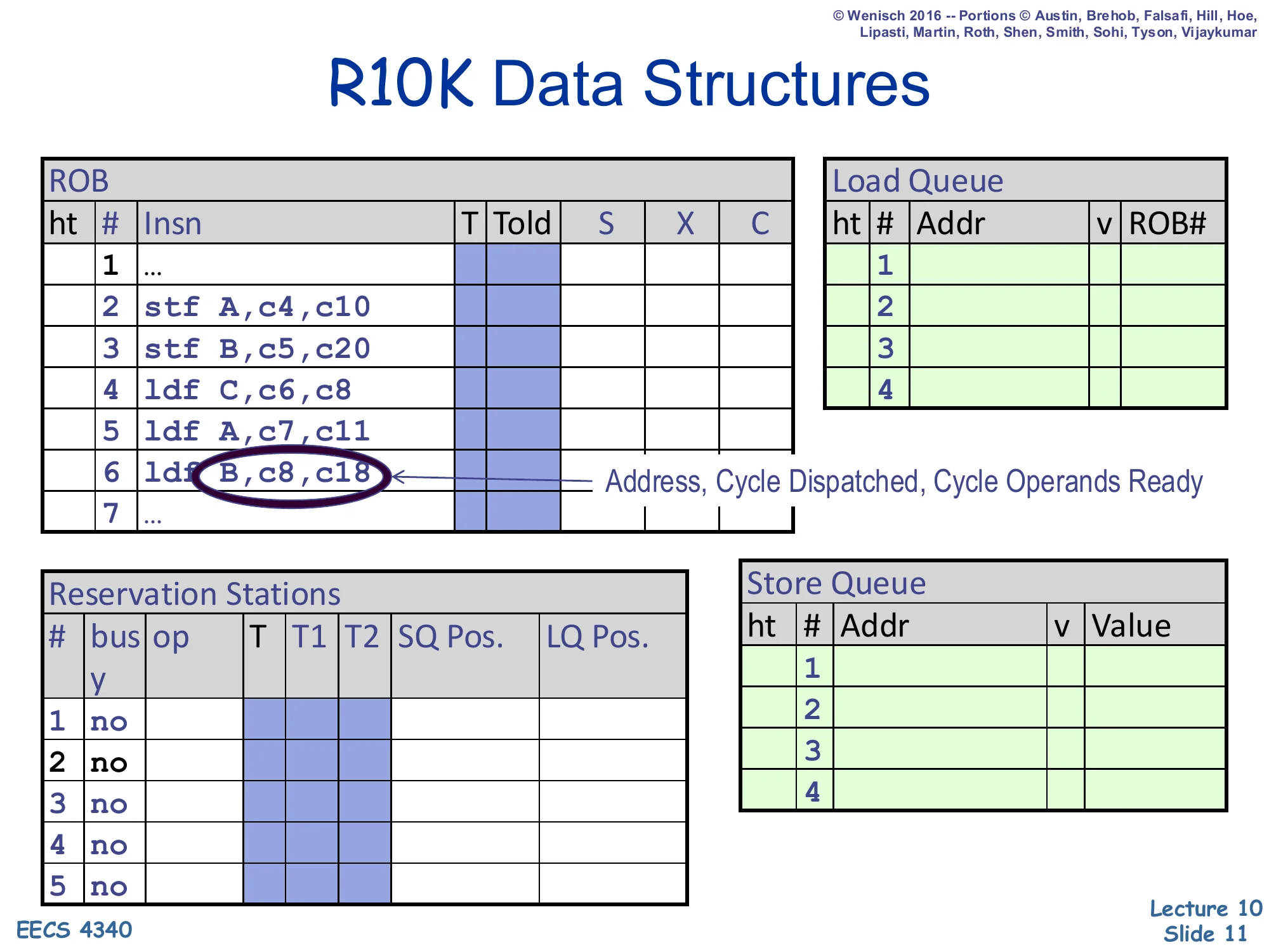
R10K Data Structures

ROB — ht | # | Insn | T | Told | S | X | C

2  stf A, c4, c10
3  stf B, c5, c20
4  ldf C, c6, c8
5  ldf A, c7, c11
6  ldf B, c8, c18  ← Address, Cycle Dispatched, Cycle Operands Ready
7  ...

Reservation Stations — # | busy | op | T | T1 | T2 | SQ Pos. | LQ Pos.

Load Queue — ht | # | Addr | v | ROB#

Store Queue — ht | # | Addr | v | Value

This is the canonical worksheet table for the MIPS R10000 pipeline used throughout the project. The ROB tracks every in-flight instruction with its renamed destination tag $T$, the previous mapping $T_{old}$ (used for rollback), and per-stage Schedule/eXecute/Complete bits. The reservation stations hold a not-yet-issued instruction with its operand tags $T_1, T_2$ plus pointers into the SQ and LQ that a memory op needs to perform its associative searches. The split queues each hold address/value for in-flight stores and addresses + ROB# back-pointers for in-flight loads. The example highlights ldf B, c8, c18 — a load whose ROB entry records both the dispatch cycle and the operand-ready cycle, the key timestamps a student fills in when tracing OoO execution by hand.

Intelligent Load Scheduling

Slide 12

Show slide text

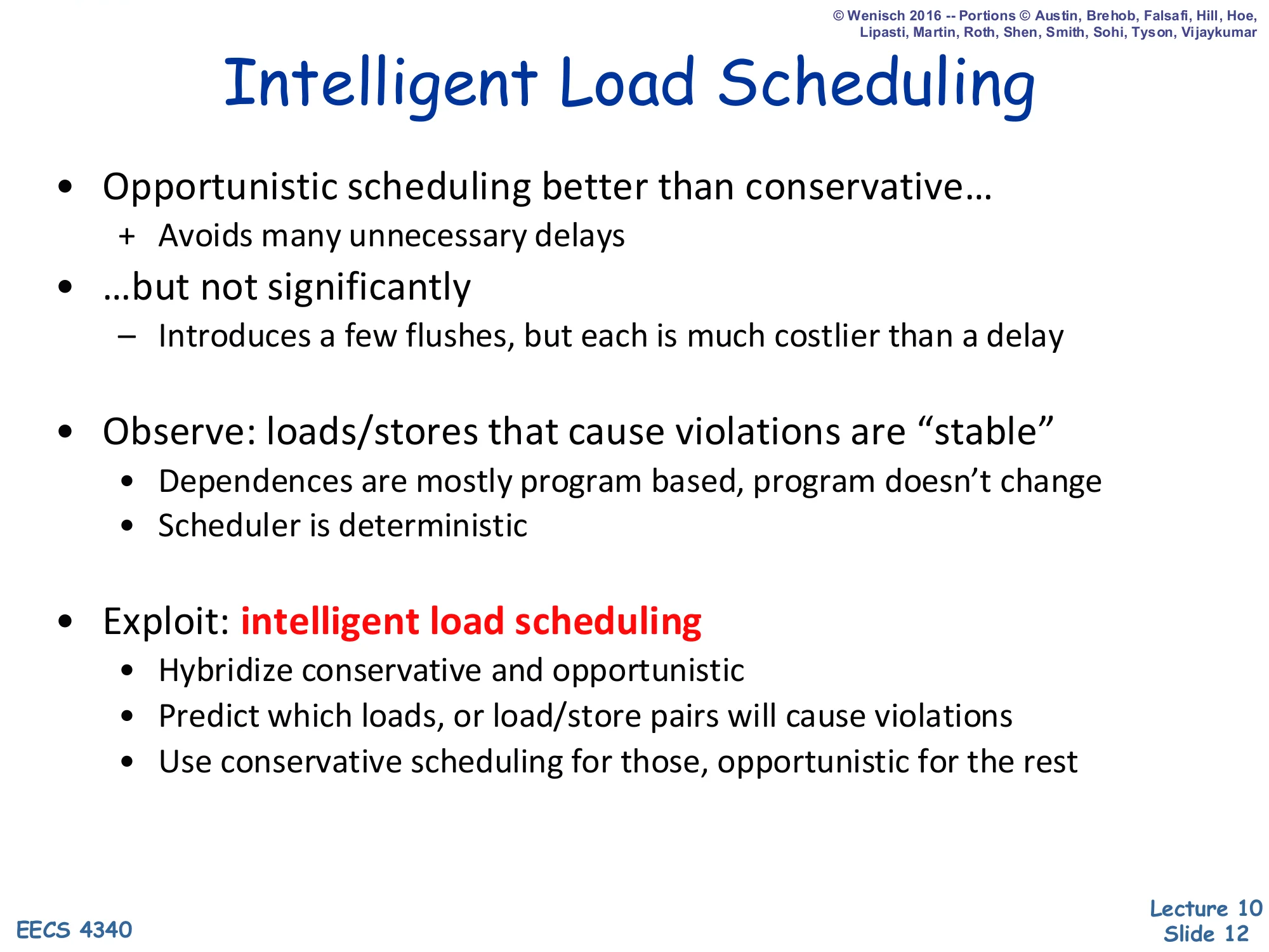
Intelligent Load Scheduling

• Opportunistic scheduling better than conservative…

  • Avoids many unnecessary delays

• …but not significantly

  • Introduces a few flushes, but each is much costlier than a delay

• Observe: loads/stores that cause violations are “stable”

  • Dependences are mostly program based, program doesn’t change
  • Scheduler is deterministic

• Exploit: intelligent load scheduling

  • Hybridize conservative and opportunistic
  • Predict which loads, or load/store pairs will cause violations
  • Use conservative scheduling for those, opportunistic for the rest

Pure speculation lets every load bypass older un-resolved stores and replay on a violation, which is fast on average but pays a full pipeline flush each time it guesses wrong. Pure conservatism waits until every older store address is known and avoids flushes but loses memory-level parallelism. The lecture’s empirical observation is that violations cluster on a small set of stable load/store pairs determined by program structure, so the right answer is a hybrid: use a dependence predictor (introduced on the next slide) to flag the rare aliasing pairs and stall those loads conservatively, while letting the vast majority of loads issue speculatively. This is the same philosophy as branch prediction — predict the rare bad outcome rather than always pay the worst-case cost — and it sets up the discussion of Store-Sets on slide 13.

Memory Dependence Prediction

Slide 13

Show slide text

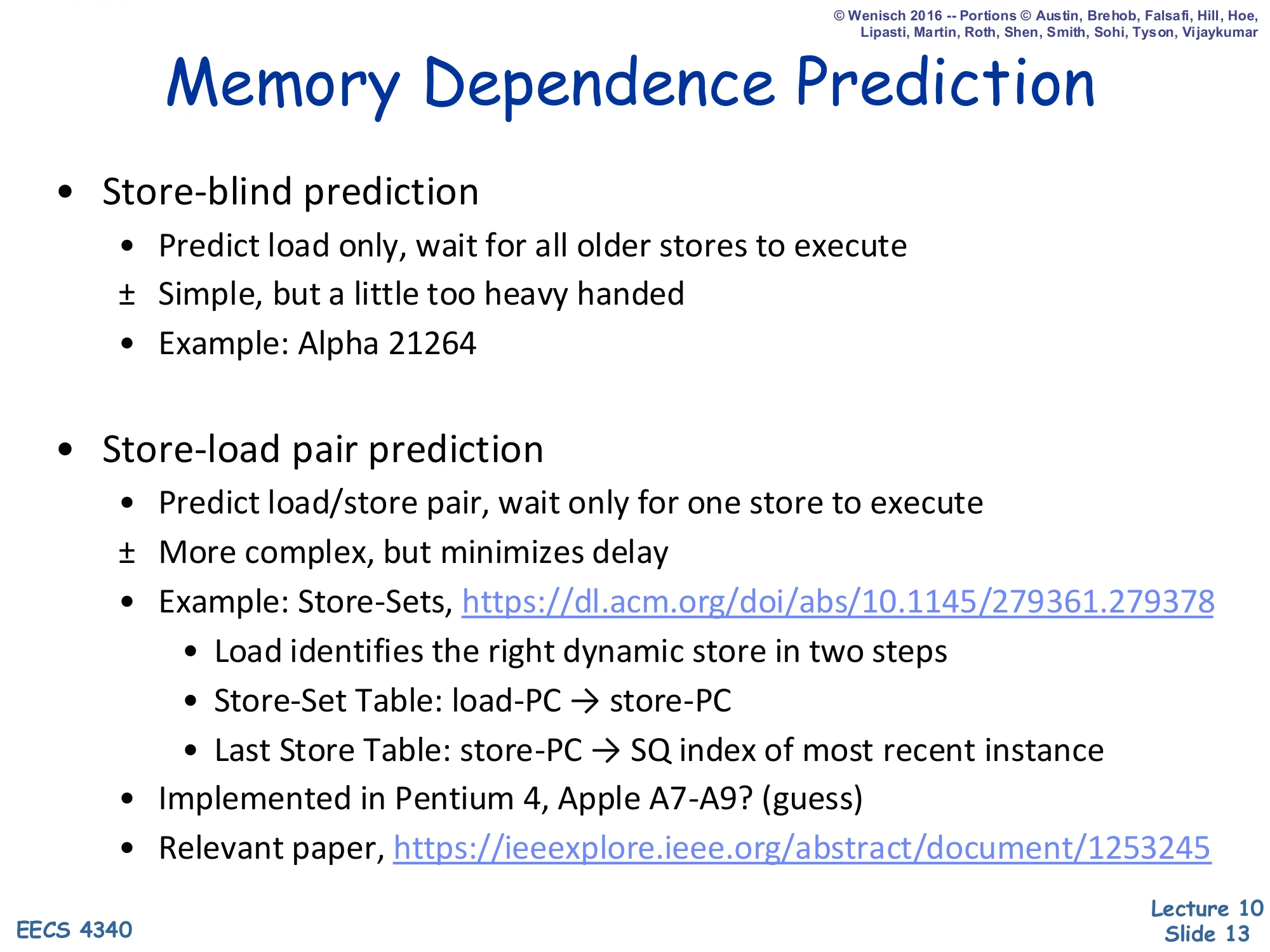
Memory Dependence Prediction

• Store-blind prediction

  • Predict load only, wait for all older stores to execute
  • ± Simple, but a little too heavy handed
  • Example: Alpha 21264

• Store-load pair prediction

  • Predict load/store pair, wait only for one store to execute
  • ± More complex, but minimizes delay
  • Example: Store-Sets, https://dl.acm.org/doi/abs/10.1145/279361.279378
    • Load identifies the first dynamic store in two steps
    • Store-Set Table: load-PC → store-PC
    • Last Store Table: store-PC → SQ index of most recent instance
  • Implemented in Pentium 4, Apple A7-A9? (guess)
  • Relevant paper, https://ieeexplore.ieee.org/abstract/document/1253245

This slide presents two granularities of memory-dependence prediction. Store-blind prediction simply marks an offending load as risky and forces it to wait for every older store to resolve — easy hardware, but it overshoots because the load only really conflicts with one store. Store-load pair prediction, exemplified by Chrysos & Emer’s Store-Sets, narrows the wait to just the specific older store the load actually aliases with, restoring most of the memory-level parallelism. Store-Sets identifies that store in two indirections: a Store-Set Table maps load PC to a store PC, and a Last Store Table maps that store PC to the store queue index of its most recent dynamic instance. The slide attributes store-blind to the Alpha 21264 and a Store-Sets-style design to the Pentium 4 and (speculatively) the Apple A7–A9. The whole structure is the memory-disambiguation half of the load/store queue.

Recap Summary

Slide 14

Show slide text

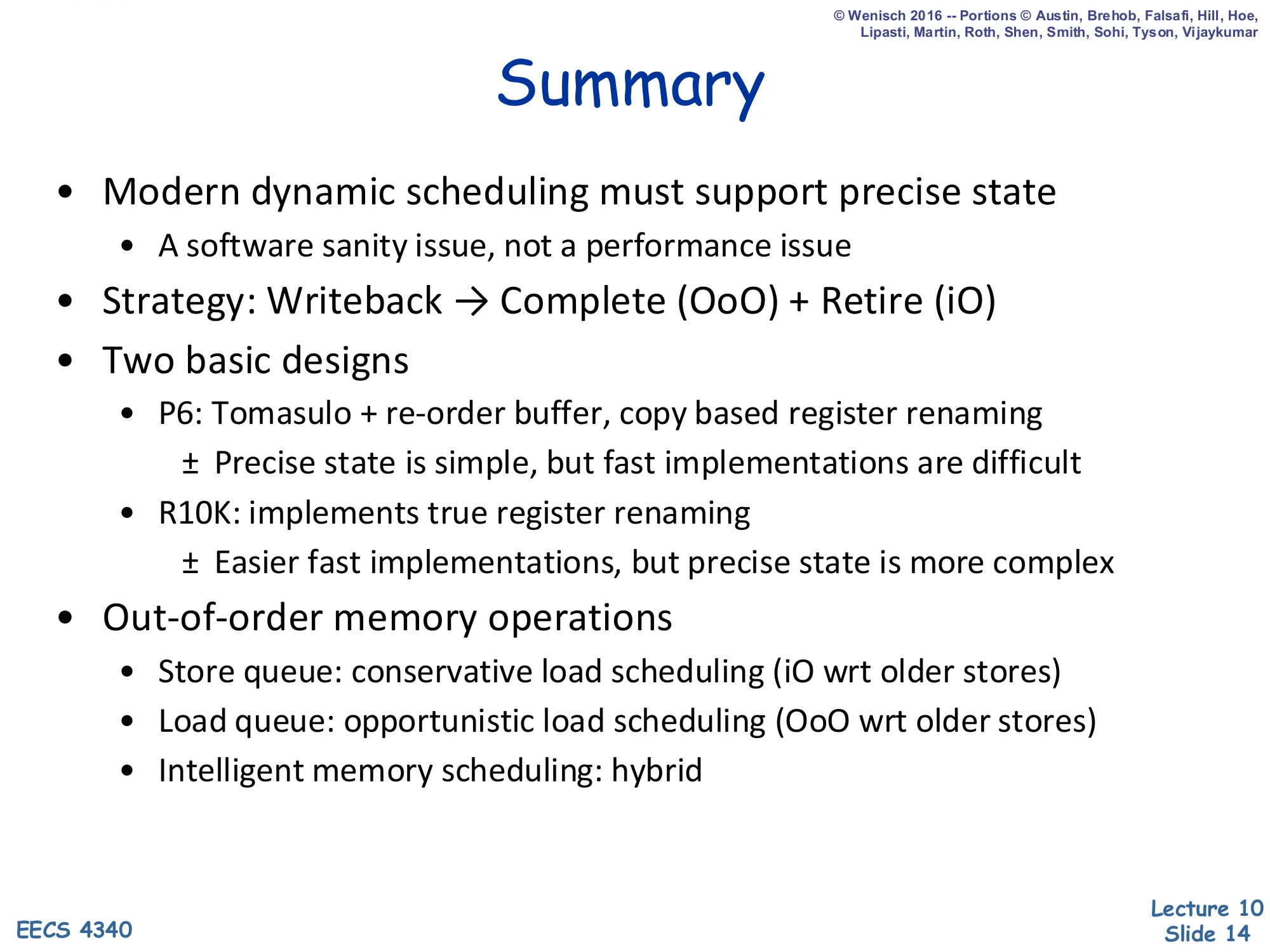
Summary

• Modern dynamic scheduling must support precise state
  • A software sanity issue, not a performance issue
• Strategy: Writeback → Complete (OoO) + Retire (iO)
• Two basic designs
  • P6: Tomasulo + re-order buffer, copy based register renaming
    • ± Precise state is simple, but fast implementations are difficult
  • R10K: implements true register renaming
    • ± Easier fast implementations, but precise state is more complex
• Out-of-order memory operations
  • Store queue: conservative load scheduling (iO wrt older stores)
  • Load queue: opportunistic load scheduling (OoO wrt older stores)
  • Intelligent memory scheduling: hybrid

The recap closes the memory-scheduling thread with the two-phase OoO completion strategy that supports precise state: instructions complete out of order at the writeback stage and then retire in order from the ROB head. Two industrial reference designs split the design space — the Pentium Pro (“P6”) layers a reorder buffer on top of Tomasulo and uses copy-based renaming, making precise state easy but fast bypass paths complex; the MIPS R10000 instead implements true register renaming into a unified physical register file, which simplifies bypass at the cost of more complex precise-state recovery. For memory operations, the store queue enforces conservative in-order behavior with respect to older stores, while a load queue enables opportunistic out-of-order issue, and intelligent memory scheduling combines both with a dependence predictor.

Branch Prediction

Slide 15

Flow Path Model of CPU

Slide 16

Show slide text

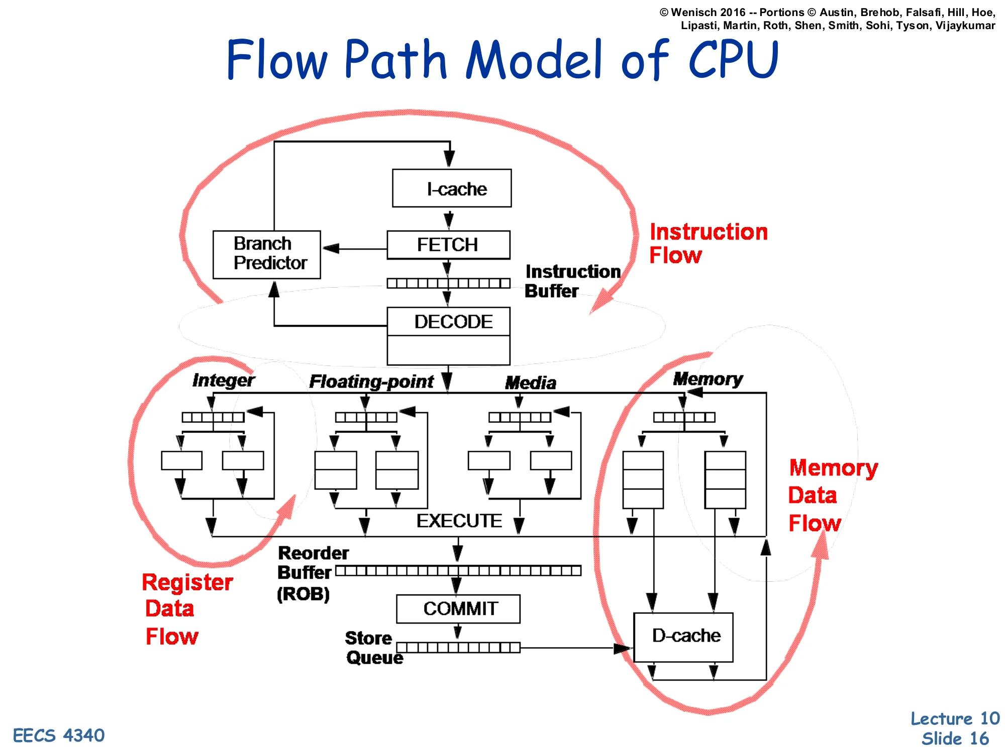
Flow Path Model of CPU

Three concurrent flows in a modern CPU:

• Instruction Flow: I-cache → Fetch → (Branch Predictor) → Instruction Buffer → Decode
• Register Data Flow: Decode → Integer/FP/Media issue queues → Execute → ROB → Commit
• Memory Data Flow: Execute → Store Queue → D-cache → Commit

This is Shen & Lipasti’s classic three-flow CPU diagram. Instruction flow loops between fetch and decode and is the flow that branches disrupt — when a branch is fetched, the branch predictor must immediately tell the front end where to go next, otherwise fetch stalls. Register data flow moves operands from decode through the issue queues, through the functional units, into the ROB, and out at commit; this is the body of out-of-order execution. Memory data flow runs in parallel, taking computed addresses through the store queue and D-cache. The lecture’s transition from memory scheduling to branch prediction is signalled by this diagram: the front-end instruction-flow loop is now the bottleneck, and the rest of the lecture is dedicated to keeping it fed.

Instruction Fetch Buffer

Slide 17

Show slide text

Instruction Fetch Buffer

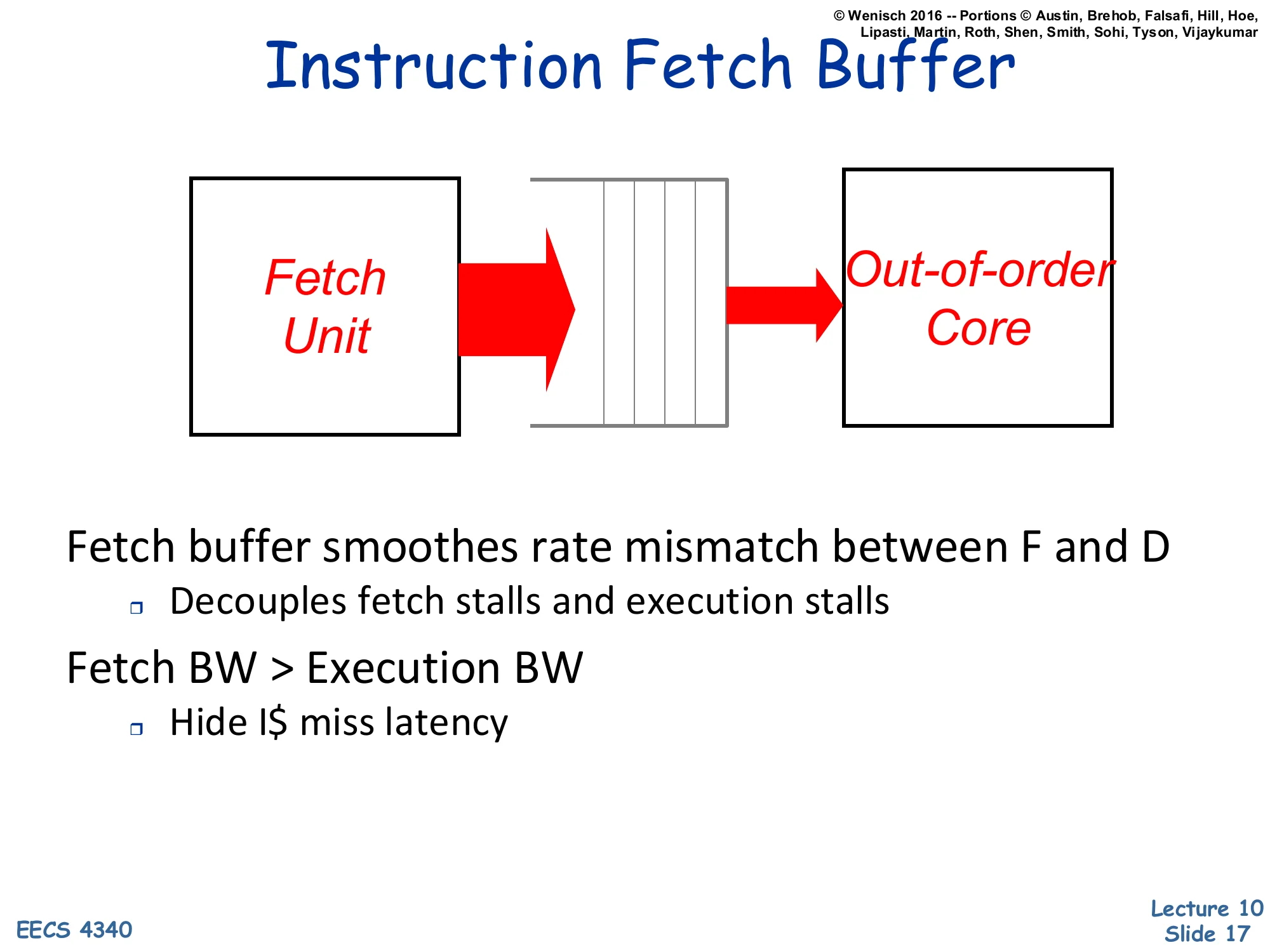
Fetch Unit → [Instruction Fetch Buffer] → Out-of-order Core

Fetch buffer smoothes rate mismatch between F and D

• Decouples fetch stalls and execution stalls

Fetch BW > Execution BW

• Hide I$ miss latency

A fetch buffer between the front-end fetch unit and the OoO core acts as a slack queue that absorbs short-term rate mismatches between the two pipelines. When an I-cache miss stalls fetch, the OoO core can keep draining instructions from the buffer, and conversely when the back end stalls (e.g., on a long-latency load), the front end keeps filling the buffer. The design rule of thumb is to provision more fetch bandwidth than peak execution bandwidth so the buffer mostly stays full and absorbs occasional miss bubbles. Branches threaten this whole scheme because every taken branch redirects fetch and can drain the buffer in one cycle, which is why front-end performance hinges on accurate branch prediction.

Review of Branches

Slide 18

Show slide text

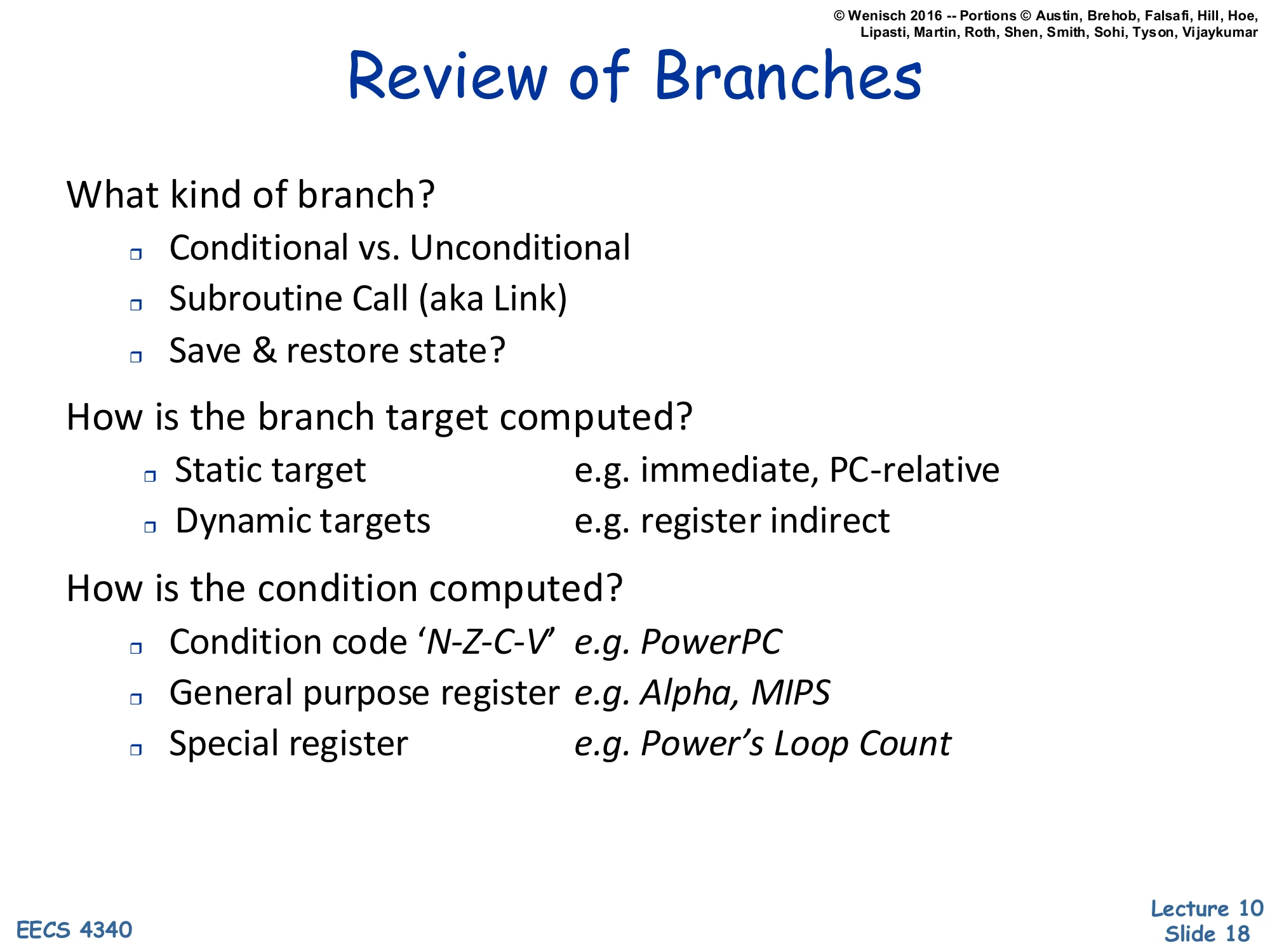
Review of Branches

What kind of branch?

• Conditional vs. Unconditional
• Subroutine Call (aka Link)
• Save & restore state?

How is the branch target computed?

• Static target — e.g. immediate, PC-relative
• Dynamic targets — e.g. register indirect

How is the condition computed?

• Condition code ‘N-Z-C-V’ — e.g. PowerPC
• General purpose register — e.g. Alpha, MIPS
• Special register — e.g. Power’s Loop Count

Branches are not a single class — they vary along three independent axes that all matter for prediction. The first axis is kind: conditional branches need direction prediction; unconditional jumps and calls only need target prediction; calls additionally interact with the return-address stack. The second axis is target computation: a static target (PC-relative immediate) is fixed at link time and is easy to predict because it never changes for a given PC, whereas a dynamic target (register indirect) can vary at every dynamic instance — virtual function calls, function-pointer indirection, and computed-goto switches. The third axis is condition computation: condition-code bits like N/Z/C/V (PowerPC), a general-purpose register comparison (Alpha, MIPS), or a dedicated counter register. These distinctions explain why a BTB alone is not enough — it predicts targets but not conditions — which motivates the separate direction predictor introduced later.

Condition Resolution

Slide 19

Show slide text

Condition Resolution

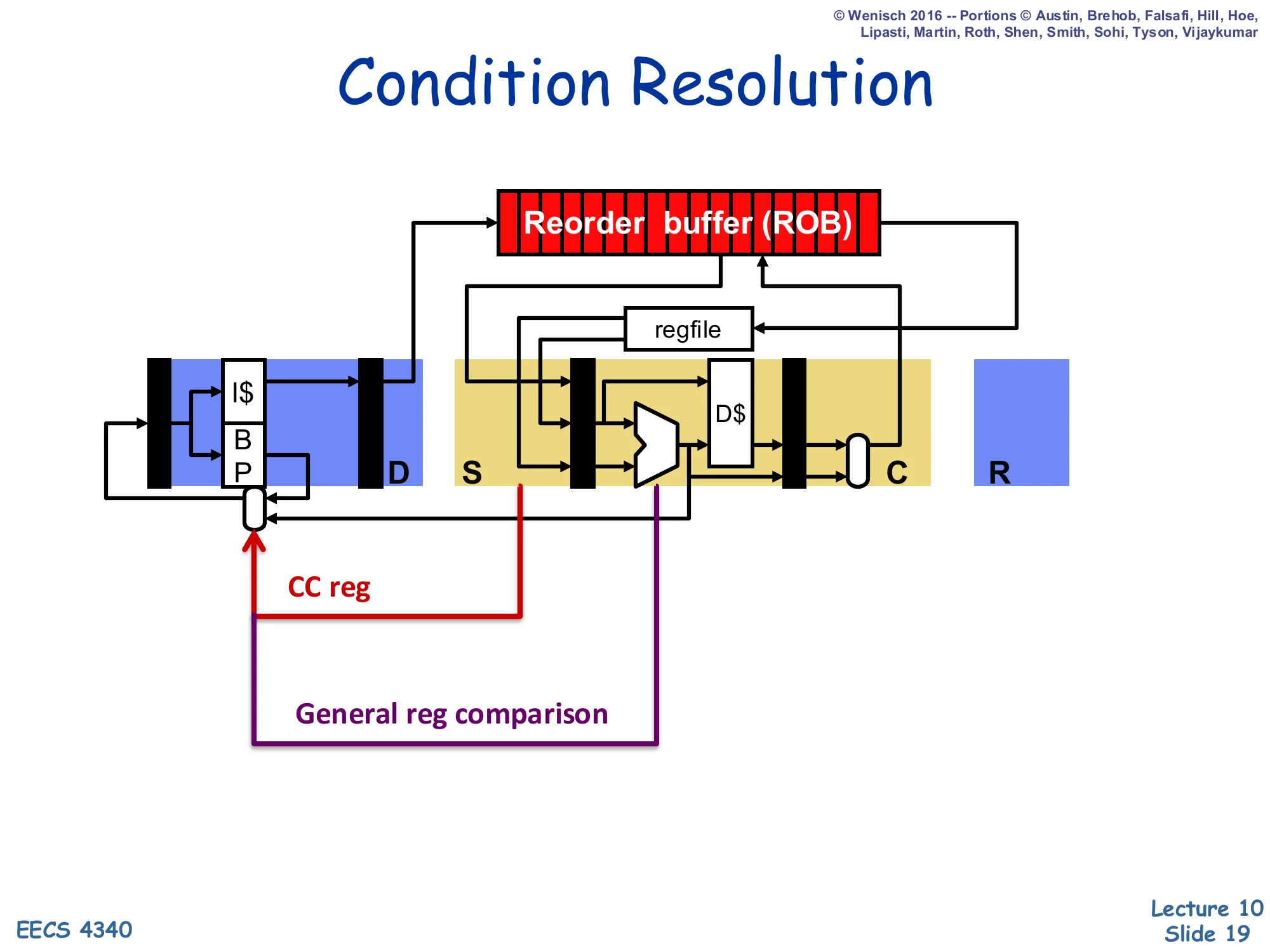
Diagram: pipeline stages D / S / C / R with ROB and regfile feeding back to the BP in fetch.

• CC reg path: condition-code register feeds back to the BP
• General reg comparison path: ALU output (e.g., compare result) feeds back to the BP

This pipeline diagram shows where a conditional branch’s outcome is actually computed and how that outcome reaches the front end to redirect fetch on a misprediction. Two physical paths exist: the CC-reg path (red) is a short read of the condition-code register taken at issue/select time on architectures like PowerPC, and the general-register-comparison path (purple) is the ALU output of an explicit comparison on Alpha/MIPS-style ISAs that goes through execute before reaching the branch resolution point. In either case, the key observation is that the branch direction is not known until somewhere in execute or commit, while fetch needs to keep going every cycle — this gap between when the branch is fetched and when its outcome is resolved is exactly the misprediction penalty window the rest of the lecture seeks to minimize.

Target Address Calculation

Slide 20

Show slide text

Target Address Calculation

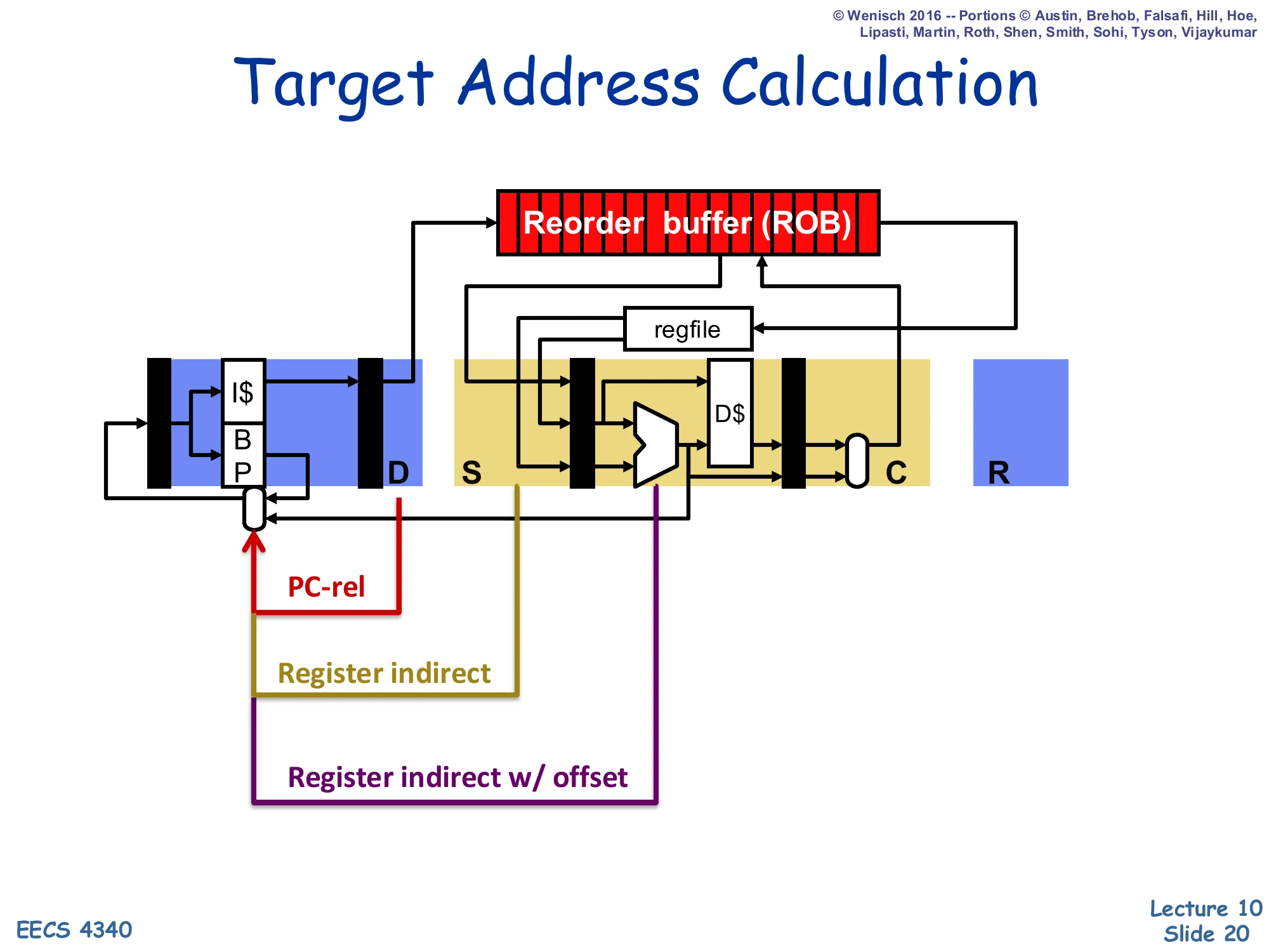
Three target-computation paths shown feeding back to the BP in fetch:

• PC-rel (red): adder in fetch/decode produces the target
• Register indirect (gold): register-file read at issue produces the target
• Register indirect w/ offset (purple): ALU adds register + offset

Where the target of a branch becomes available in the pipeline depends on how it is computed. PC-relative branches (most direct conditional and unconditional jumps) compute their target with a small adder in fetch/decode, so the target is known almost immediately and a BTB hit can be verified quickly. Register-indirect branches (returns, function pointers, virtual calls) cannot compute their target until the source register is read — that may be at issue time, much later than fetch. Register-indirect-with-offset (used for jump tables and some indirect calls) waits even longer because the ALU must add the offset. The BTB exists precisely so the front end does not stall waiting for these later resolution points; it provides a speculative target the cycle the branch is fetched.

What's So Bad About Branches?

Slide 21

Show slide text

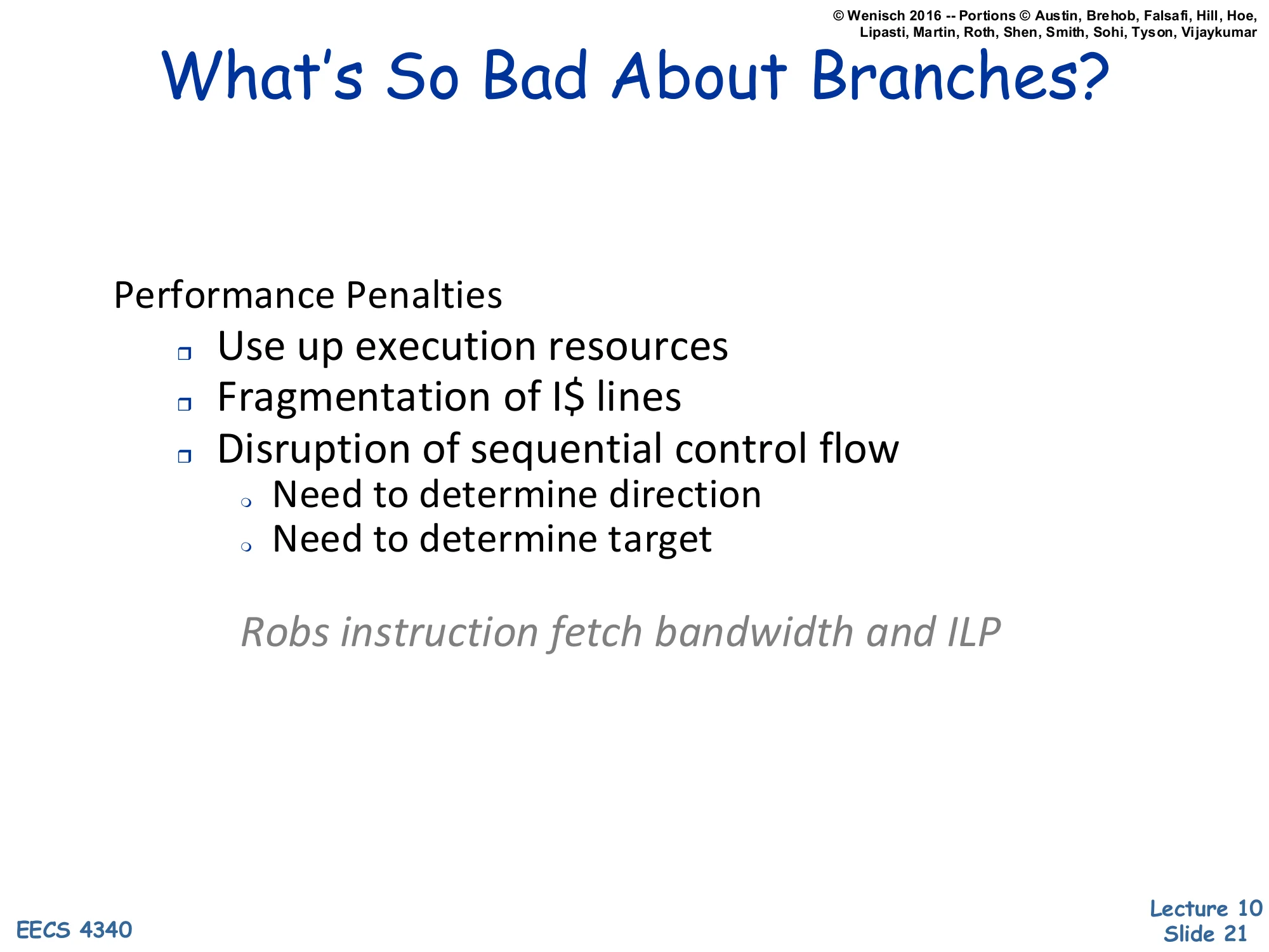
What’s So Bad About Branches?

Performance Penalties

• Use up execution resources
• Fragmentation of I$ lines
• Disruption of sequential control flow
  • Need to determine direction
  • Need to determine target

Robs instruction fetch bandwidth and ILP

Branches hurt performance in three distinct ways. First, they consume an issue slot and a functional unit even when they have no observable side effect on registers, so they directly reduce useful IPC. Second, taken branches create fragmentation in the instruction cache because the next sequential bytes after a taken branch are wasted; a 16-byte fetch line that contains a taken branch in the middle effectively delivers only the bytes up to the branch. Third — and most importantly — branches disrupt sequential control flow: until both direction and target are known, fetch cannot reliably continue, so they directly attack the front end’s ability to keep the OoO core fed with instructions. Together these three effects rob both fetch bandwidth and instruction-level parallelism, which is why branch prediction is the highest-leverage front-end optimization.

Penalty of Branch Misprediction

Slide 22

Show slide text

Penalty of Branch Misprediction

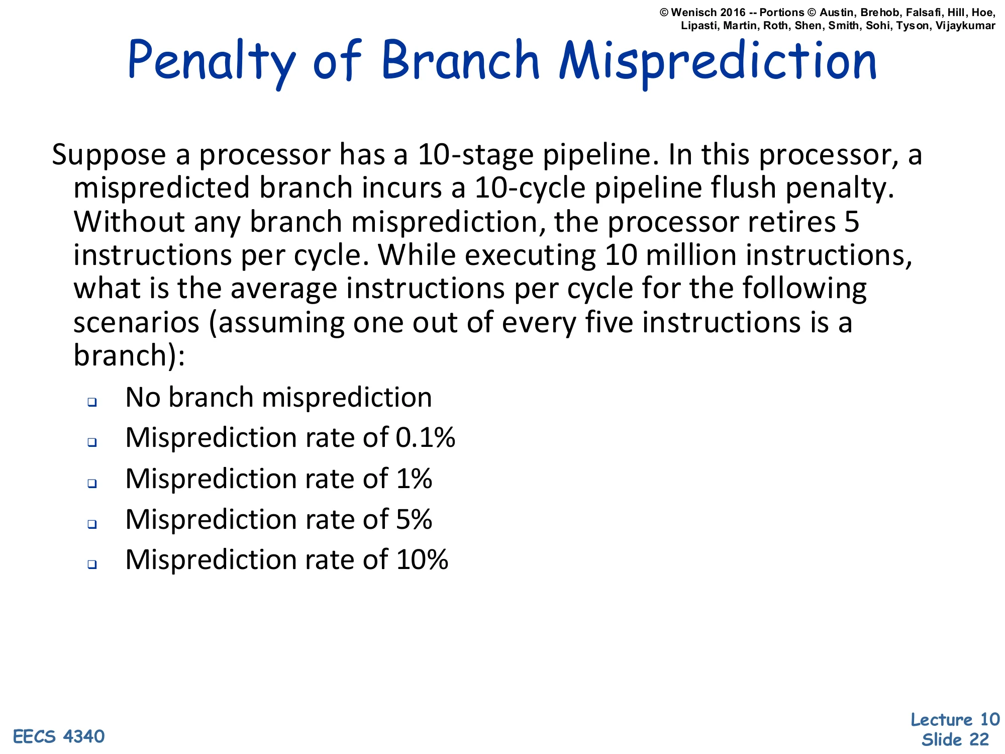
Suppose a processor has a 10-stage pipeline. In this processor, a mispredicted branch incurs a 10-cycle pipeline flush penalty. Without any branch misprediction, the processor retires 5 instructions per cycle. While executing 10 million instructions, what is the average instructions per cycle for the following scenarios (assuming one out of every five instructions is a branch):

• No branch misprediction
• Misprediction rate of 0.1%
• Misprediction rate of 1%
• Misprediction rate of 5%
• Misprediction rate of 10%

This worked exam problem quantifies why even a small misprediction rate is catastrophic in a deep pipeline. With $N=10^7$ instructions, branch frequency $f_b=0.2$, peak IPC $5$, and misprediction penalty $P=10$ cycles, the baseline cycles is $N/5 = 2 \cdot 10^6$. Each misprediction adds $P=10$ flush cycles, so total cycles $= N/5 + N \cdot f_b \cdot p_m \cdot P$ where $p_m$ is the misprediction rate. The IPC is then $\text{IPC} = \frac{N}{N/5 + N f_b p_m P} = \frac{1}{0.2 + 0.2 \cdot p_m \cdot 10} = \frac{1}{0.2(1 + 10 p_m)}.$ Plugging in: at $p_m=0$, IPC=5; at $0.1\%$, IPC≈4.95; at $1\%$, IPC≈4.55; at $5\%$, IPC≈3.33; at $10\%$, IPC=2.5. A 10% misprediction rate halves IPC — exactly why the Iron Law makes branch prediction worth significant area and power.

Branch Prediction (Static vs Dynamic)

Slide 23

Show slide text

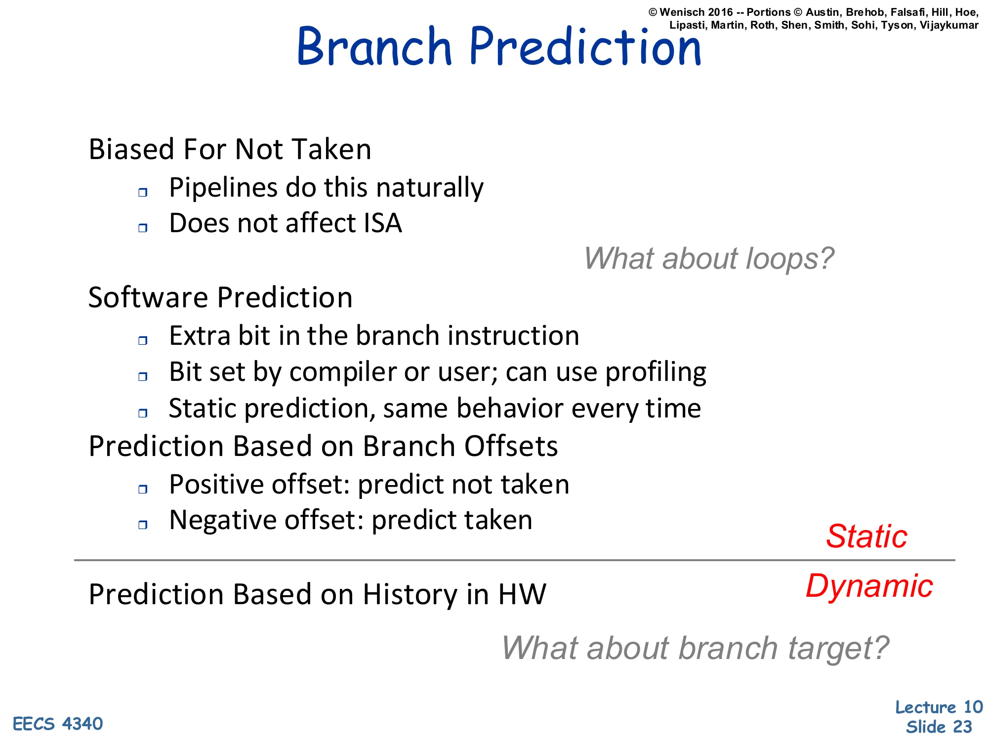
Branch Prediction

Biased For Not Taken (Static)

• Pipelines do this naturally
• Does not affect ISA

What about loops?

Software Prediction (Static)

• Extra bit in the branch instruction
• Bit set by compiler or user; can use profiling
• Static prediction, same behavior every time

Prediction Based on Branch Offsets (Static)

• Positive offset: predict not taken
• Negative offset: predict taken

— Static / Dynamic line —

Prediction Based on History in HW (Dynamic)

What about branch target?

This slide enumerates four points along a static-to-dynamic spectrum of branch prediction. The cheapest static rule is predict not-taken: it costs nothing because the natural sequential PC increment is already correct on a not-taken outcome — but it loses on every backward loop branch, which is taken on every iteration except the last. Software prediction adds one hint bit per branch instruction that the compiler sets from profile data; it survives across runs but cannot adapt. Offset-based prediction encodes a useful heuristic — backward (negative offset) branches are usually loops and likely taken, forward (positive offset) branches are usually error paths and likely not taken — and recovers most of the loop-vs-error-path benefit without ISA changes. The static-dynamic line then introduces history-based hardware prediction, which adapts at runtime. The closing question — what about branch target? — sets up the BTB discussion two slides later.

Dynamic Branch Prediction

Slide 24

Show slide text

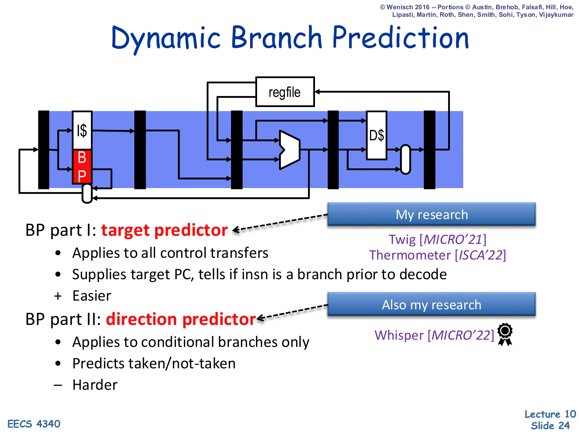
Dynamic Branch Prediction

Diagram: a BP block in the fetch stage produces next-PC each cycle.

BP part I: target predictor

• Applies to all control transfers
• Supplies target PC, tells if insn is a branch prior to decode
• • Easier

BP part II: direction predictor

• Applies to conditional branches only
• Predicts taken/not-taken
• − Harder

Dynamic branch prediction cleanly factors into two cooperating subproblems. The target predictor — a BTB in most designs — is queried with the current PC every fetch cycle and answers two questions at once: “is this byte the start of a control-transfer instruction?” and “if so, where does it go (assuming taken)?”. This is comparatively easy because targets of direct branches are constants and even most indirect targets are stable across calls. The direction predictor is harder: it must guess whether each conditional branch will go taken or not-taken on this dynamic instance, with no help from the static instruction encoding. The lecture spends roughly slides 25–28 on the target side (BTB and RAS) and slides 29 onward on the harder direction-prediction problem (BHT, 2-bit counters, correlated/two-level, GShare, hybrid, TAGE).

Branch Target Buffer

Slide 25

Show slide text

Branch Target Buffer

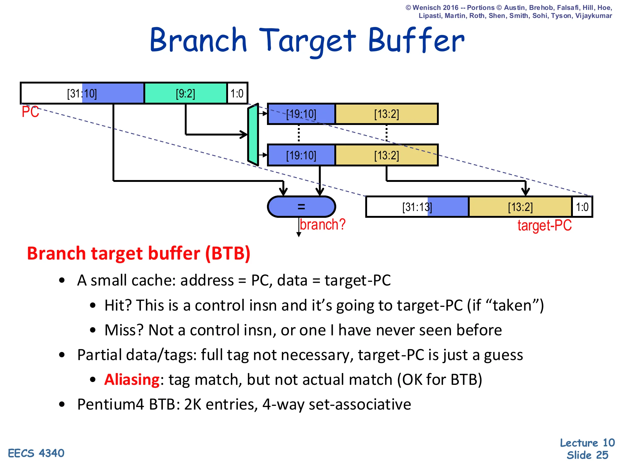
Diagram: PC[31:10] | PC[9:2] | 1:0 indexes a set; each way holds tag bits [19:10] and target [13:2]. Hit raises branch? and selects target-PC = {PC[31:13], stored [13:2], 1:0}.

Branch target buffer (BTB)

• A small cache: address = PC, data = target-PC
  • Hit? This is a control insn and it’s going to target-PC (if “taken”)
  • Miss? Not a control insn, or one I have never seen before
• Partial data/tags: full tag not necessary, target-PC is just a guess
  • Aliasing: tag match, but not actual match (OK for BTB)
• Pentium 4 BTB: 2K entries, 4-way set-associative

The BTB is a small set-associative cache indexed by the low PC bits whose tag is a slice of the upper PC bits and whose data is the predicted target PC. Because the BTB is speculative — every prediction is verified later in the pipeline — it can use partial tags and partial targets, exploiting the high entropy of real PCs to keep the storage small without much loss in accuracy. Aliasing (two different PCs with the same partial tag) is tolerated because a wrong prediction is just a normal misprediction, recoverable by the existing flush machinery. The example sizing (Pentium 4: 2K entries, 4-way) shows the typical scale of a BTB in a desktop core. A BTB hit produces both a branch? signal (used by the front end to decide whether to redirect) and the target-PC, all in the same cycle the branch is fetched, which is what enables zero-bubble taken branches when the prediction is right.

Branch Prediction Unit (BPU) Overview

Slide 26

Show slide text

Branch Prediction Unit

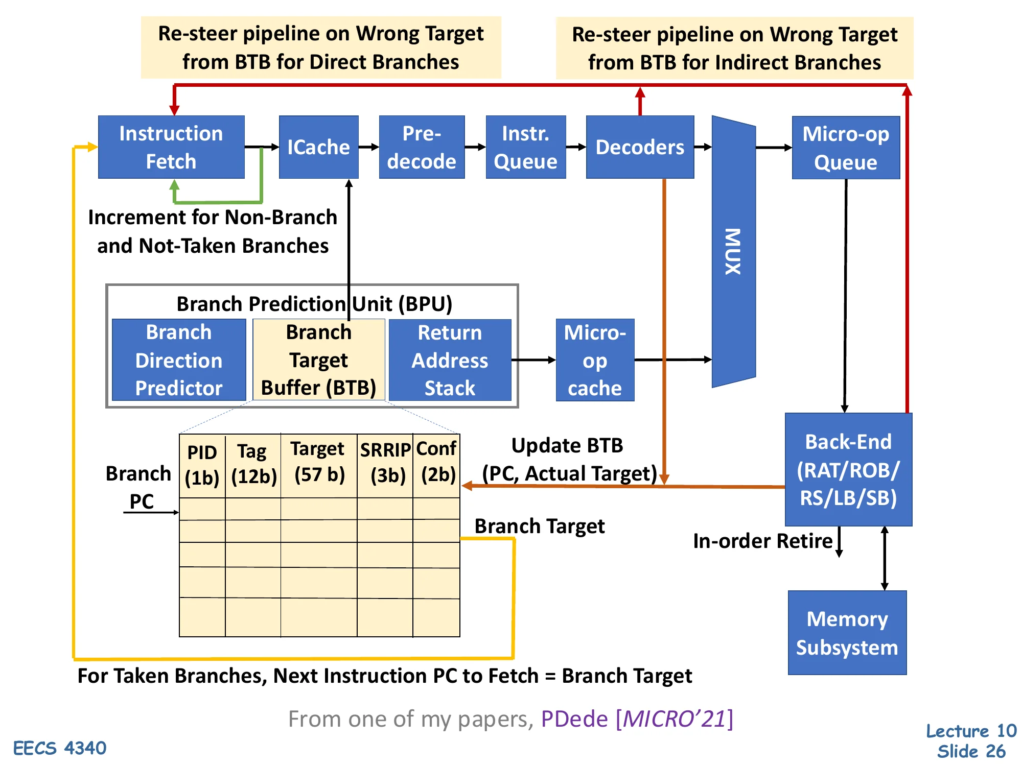
Front-end pipeline: Instruction Fetch → ICache → Pre-decode → Instr. Queue → Decoders → MUX → Micro-op Queue → Back-End (RAT/ROB/RS/LB/SB) → Memory Subsystem.

Branch Prediction Unit (BPU) sits beside fetch and contains:

• Branch Direction Predictor
• Branch Target Buffer (BTB) — entry: PID(1b), Tag(12b), Target(57b), SRRIP(3b), Conf(2b)
• Return Address Stack
• Micro-op cache

For taken branches, next instruction PC to fetch = Branch Target. Increment for non-branch and not-taken branches. Update BTB (PC, Actual Target) on misprediction; re-steer pipeline on wrong target from BTB for both direct and indirect branches.

From PDede [MICRO’21]

This block diagram is a modern Intel-class front end. The Branch Prediction Unit is queried in parallel with the I-cache so that target and direction predictions are available the same cycle the bytes return. The BPU bundles three structures: a BTB for direct/indirect targets (with example fields PID, partial tag, 57-bit target, SRRIP replacement, and a confidence counter), a return-address stack for return targets, and a separate direction predictor for conditional branches. A separate micro-op cache short-circuits decode for hot loops. Re-steering happens at multiple points: a BTB miss or wrong target detected after pre-decode redirects the pipeline immediately; an indirect branch whose actual target differs from the BTB prediction redirects much later. The 2-bit confidence field is the kind of mechanism used by recent research (e.g., Twig, Thermometer, PDede) to reduce wasted re-steers on low-confidence predictions.

Why Does a BTB Work?

Slide 27

Show slide text

Why Does a BTB Work?

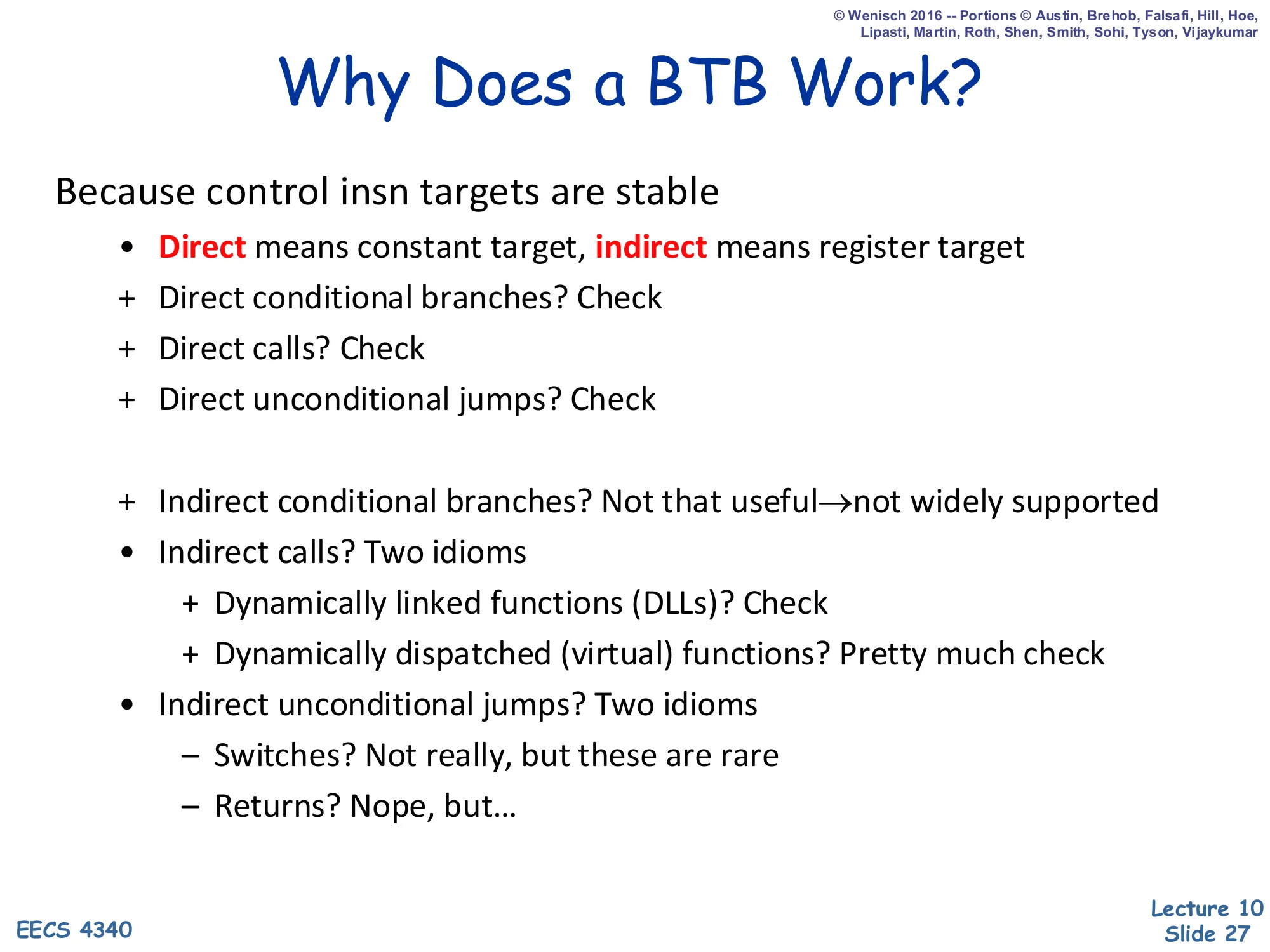
Because control insn targets are stable

• Direct means constant target, indirect means register target

• • Direct conditional branches? Check
• • Direct calls? Check
• • Direct unconditional jumps? Check
• • Indirect conditional branches? Not that useful → not widely supported

• Indirect calls? Two idioms

  • • Dynamically linked functions (DLLs)? Check
  • • Dynamically dispatched (virtual) functions? Pretty much check

• Indirect unconditional jumps? Two idioms

  • − Switches? Not really, but these are rare
  • − Returns? Nope, but…

The BTB only works because of empirical target stability: most control instructions, even indirect ones, hit the same target on consecutive dynamic instances. Direct branches (conditional, calls, jumps) all encode a constant offset and therefore have a single fixed target — these are perfect BTB customers. Indirect calls divide into two idioms that also work: PLT entries for dynamically-linked functions resolve to one address per program execution, and virtual-function dispatch usually has a stable type at each call site. The two idioms that don’t fit the BTB are switch/jump-tables (target genuinely varies with runtime data) and returns — a return’s target depends on the call site, so the same return PC routinely sees many different targets. Returns motivate the return-address stack, introduced on the next slide as a separate structure that mirrors call/return semantics.

Return Address Stack (RAS)

Slide 28

Show slide text

Return Address Stack (RAS)

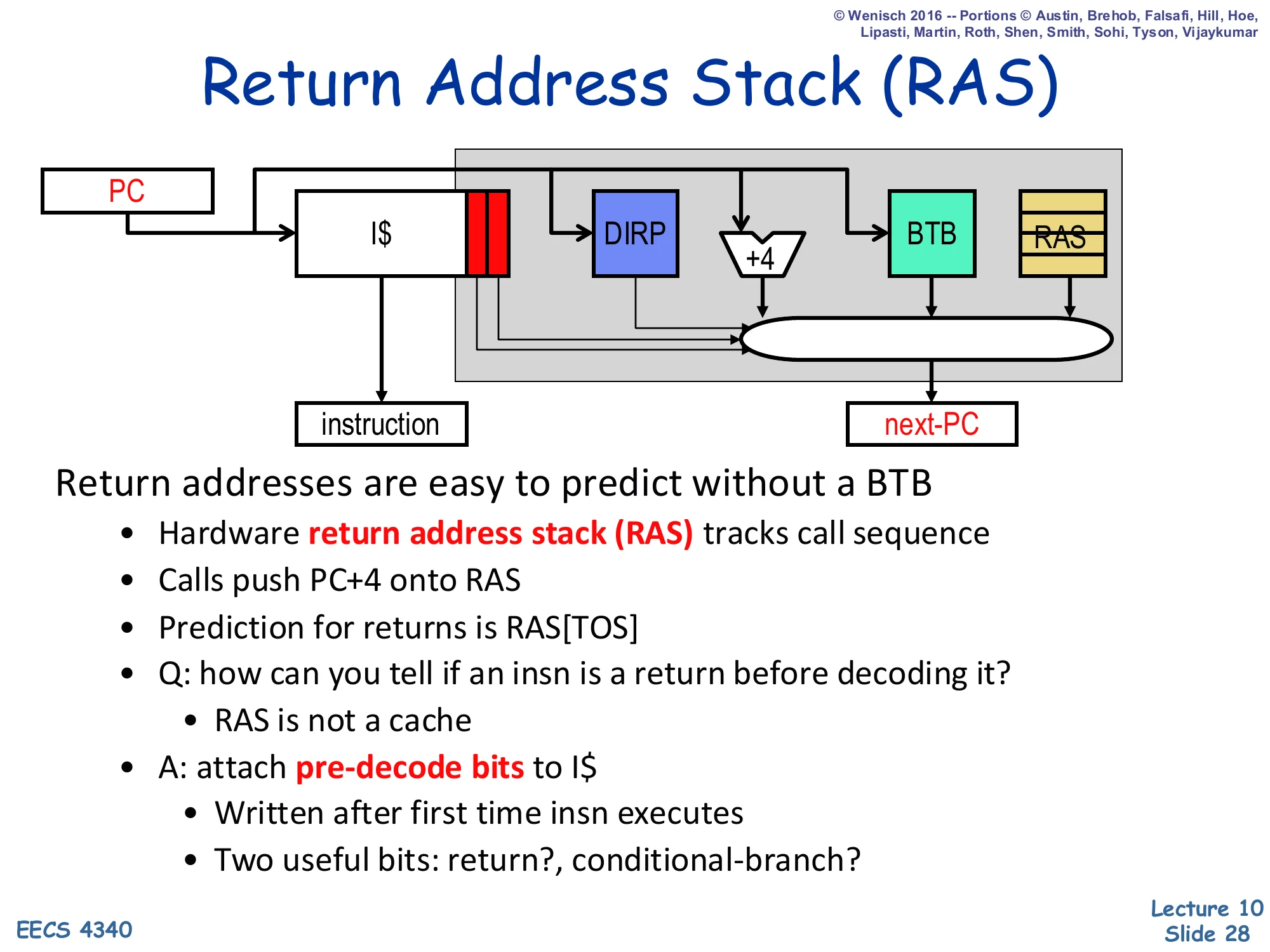
Diagram: PC indexes I$, which produces the instruction and pre-decode bits. Pre-decode bits enable DIRP, +4, BTB, and RAS in parallel. A MUX selects next-PC from {+4, DIRP, BTB, RAS}.

Return addresses are easy to predict without a BTB

• Hardware return address stack (RAS) tracks call sequence
• Calls push PC+4 onto RAS
• Prediction for returns is RAS[TOS]
• Q: how can you tell if an insn is a return before decoding it?
  • RAS is not a cache
• A: attach pre-decode bits to I$
  • Written after first time insn executes
  • Two useful bits: return?, conditional-branch?

The Return Address Stack is a tiny circular hardware stack that mirrors the program’s call/return discipline. On a call, the front end pushes $PC+4$ (the address of the instruction after the call) onto the RAS; on a return, the predicted target is just the top-of-stack entry. Because well-formed programs always pair calls with returns, this scheme reaches near-perfect accuracy on returns — a problem the BTB is hopeless at because each return PC sees many targets. The implementation question — how does fetch even know an instruction is a return before decoding it? — is solved with pre-decode bits stored alongside each I-cache line and written when the instruction first executes. Two bits suffice: return? and conditional-branch?. Because the I-cache is a real cache (subject to eviction), these bits effectively cache decode information; on a cold miss the front end falls back to slower paths.

Branch Direction Prediction (DIRP)

Slide 29

Show slide text

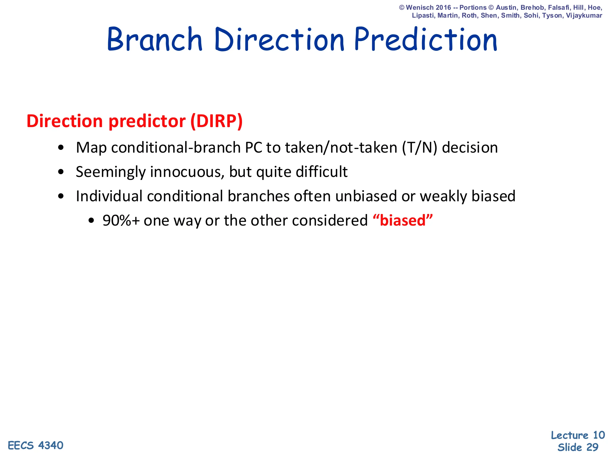
Branch Direction Prediction

Direction predictor (DIRP)

• Map conditional-branch PC to taken/not-taken (T/N) decision
• Seemingly innocuous, but quite difficult
• Individual conditional branches often unbiased or weakly biased
  • 90%+ one way or the other considered “biased”

This slide reframes the rest of the lecture as the direction-prediction problem: given a conditional-branch PC, predict T or N. The slide’s emphasis is that this is not a trivial classification task — empirically, only a fraction of conditional branches are biased (defined here as taking the same direction at least 90% of the time). The remaining unbiased branches are the ones that drive misprediction rate: a branch that flips T/N near 50/50 cannot be predicted by a memoryless rule and demands history-based predictors. The next several slides introduce successively more powerful direction predictors — single-bit BHT, 2-bit saturating counters, two-level correlated predictors, GShare, hybrid predictors, and TAGE — each of which exploits a different kind of correlation in branch outcomes.

Branch History Table (BHT)

Slide 30

Show slide text

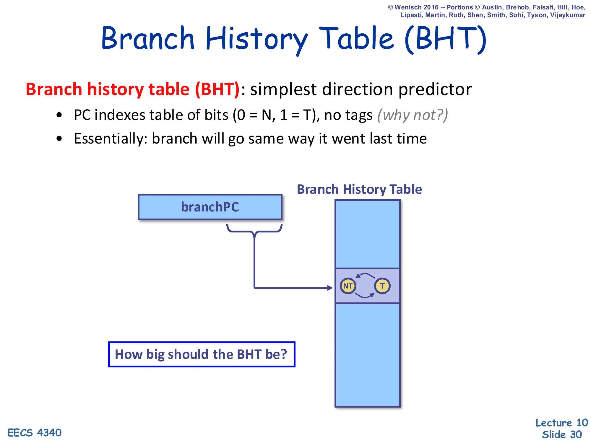
Branch History Table (BHT)

Branch history table (BHT): simplest direction predictor

• PC indexes table of bits (0 = N, 1 = T), no tags (why not?)
• Essentially: branch will go same way it went last time

Diagram: branchPC’s low bits index into the BHT; the entry is a 1-bit FSM with states NT and T.

How big should the BHT be?

The simplest direction predictor is the Branch History Table: a flat array of 1-bit entries indexed by the low bits of the branch PC, no tags at all. The entry encodes last outcome — taken or not-taken — and predicts the same direction next time. Tags are unnecessary because, like the BTB target, a wrong prediction is just an ordinary misprediction the back end will catch and fix. The size question is a design tradeoff: too small and many unrelated PCs alias to the same entry (constructive interference for biased branches, destructive for unbiased ones); too large and the table area dominates the front end. Typical real BHTs range from a few thousand to tens of thousands of entries. The next slide shows the catastrophic failure mode of this 1-bit predictor on simple inner loops.

Limitations of Simple Prediction

Slide 31

Show slide text

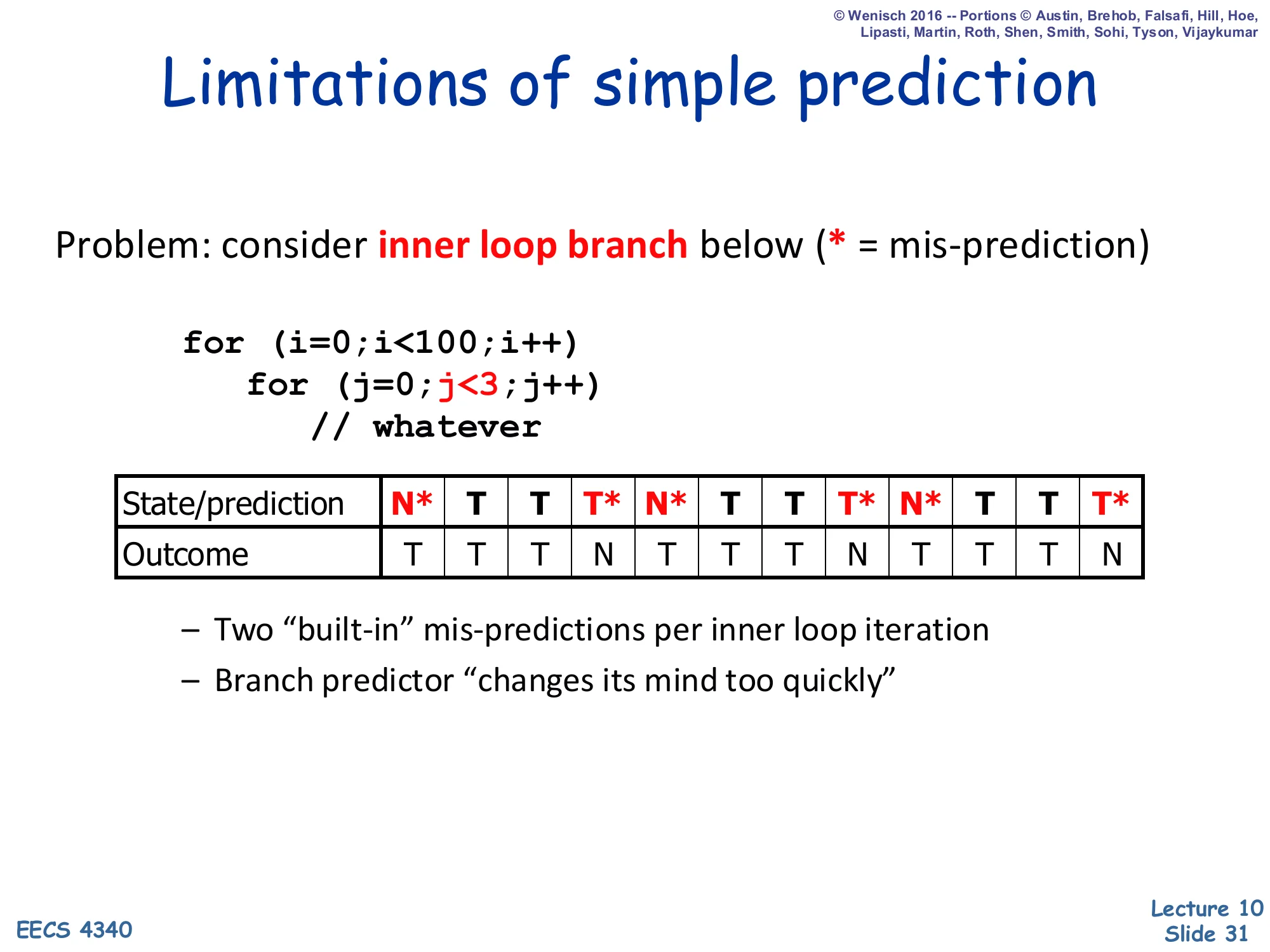
Limitations of simple prediction

Problem: consider inner loop branch below (* = mis-prediction)

for (i=0; i<100; i++)
    for (j=0; j<3; j++)
        // whatever

State/prediction: N* T T T* N* T T T* N* T T T* Outcome: T T T N T T T N T T T N

• Two “built-in” mis-predictions per inner loop iteration
• Branch predictor “changes its mind too quickly”

This slide demonstrates the pathology that motivates the 2-bit saturating counter. The inner loop for(j=0; j<3; j++) produces the repeating outcome pattern T,T,T,N — three taken iterations and one falling-out. With a 1-bit BHT, each falling-out flips the state from T to N, which then mispredicts the very next iteration of the outer loop where the branch should be predicted T again. Concretely, the slide shows two mispredictions per outer-loop iteration: one when the loop exits (T predicted but outcome is N) and one when it re-enters (N predicted but outcome is T). The diagnosis is that the predictor changes its mind too quickly — a single counter-example overrides many consistent observations. The fix on the next slide is a 2-bit hysteresis counter that requires two mispredictions before flipping, halving the mispredictions on this pattern.

Two-Bit Saturating Counters (2bc)

Slide 32

Show slide text

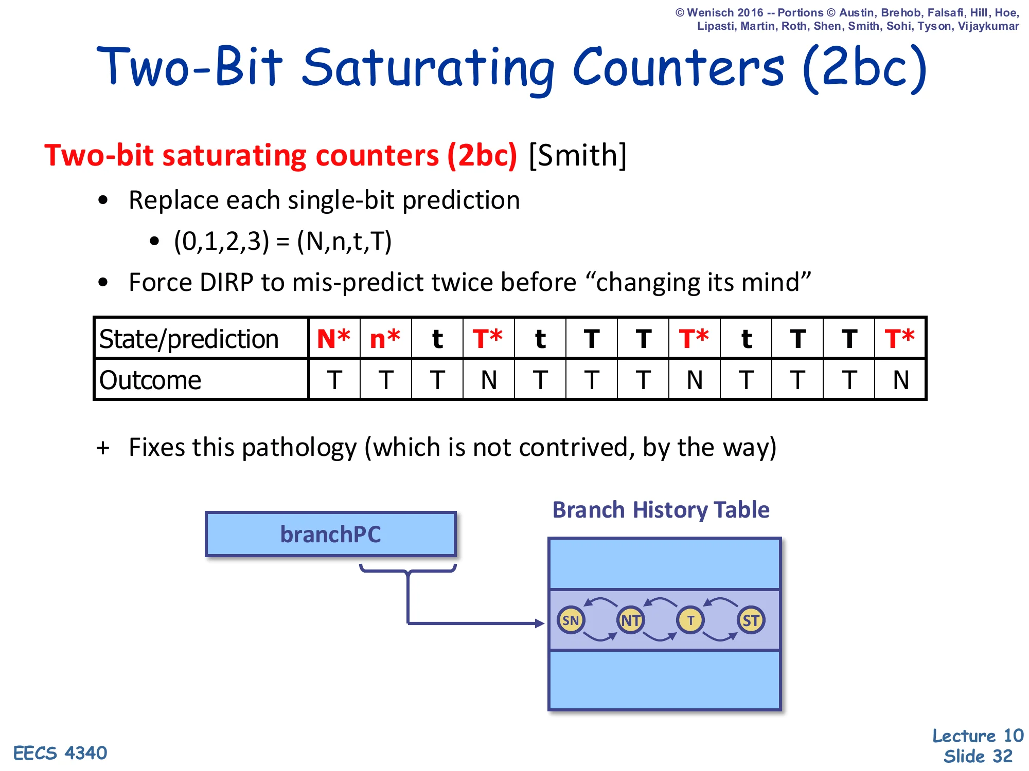
Two-Bit Saturating Counters (2bc)

Two-bit saturating counters (2bc) [Smith]

• Replace each single-bit prediction
  • $(0,1,2,3) = (N, n, t, T)$
• Force DIRP to mis-predict twice before “changing its mind”

State/prediction: N* n* t T* t T T T* t T T T* Outcome: T T T N T T T N T T T N

• Fixes this pathology (which is not contrived, by the way)

Diagram: branchPC indexes the BHT; each entry is a 4-state FSM: SN ↔ NT ↔ T ↔ ST.

Show slide text

State key: SN = strongly not-taken (00), NT = weakly not-taken (01), T = weakly taken (10), ST = strongly taken (11).

Smith’s 2-bit saturating counter (also called a bimodal predictor) is the textbook fix to the 1-bit pathology. Each entry holds a 2-bit state: strongly not-taken (00), weakly not-taken (01), weakly taken (10), strongly taken (11). The predictor outputs taken iff the high bit is 1. On a taken outcome the counter increments (saturating at 11), on not-taken it decrements (saturating at 00). The hysteresis — the counter must be wrong twice in a row before flipping its top bit — eliminates exactly the misprediction pattern from slide 31: when the inner loop falls out, the entry only moves from ST to T, still predicting taken on the next outer iteration. The slide shows the same outcome stream with at most one misprediction per pattern transition instead of two.

2-bit saturating counter FSM. Predicts taken when in T or ST.

Other Prediction Algorithms

Slide 33

Show slide text

Other Prediction Algorithms

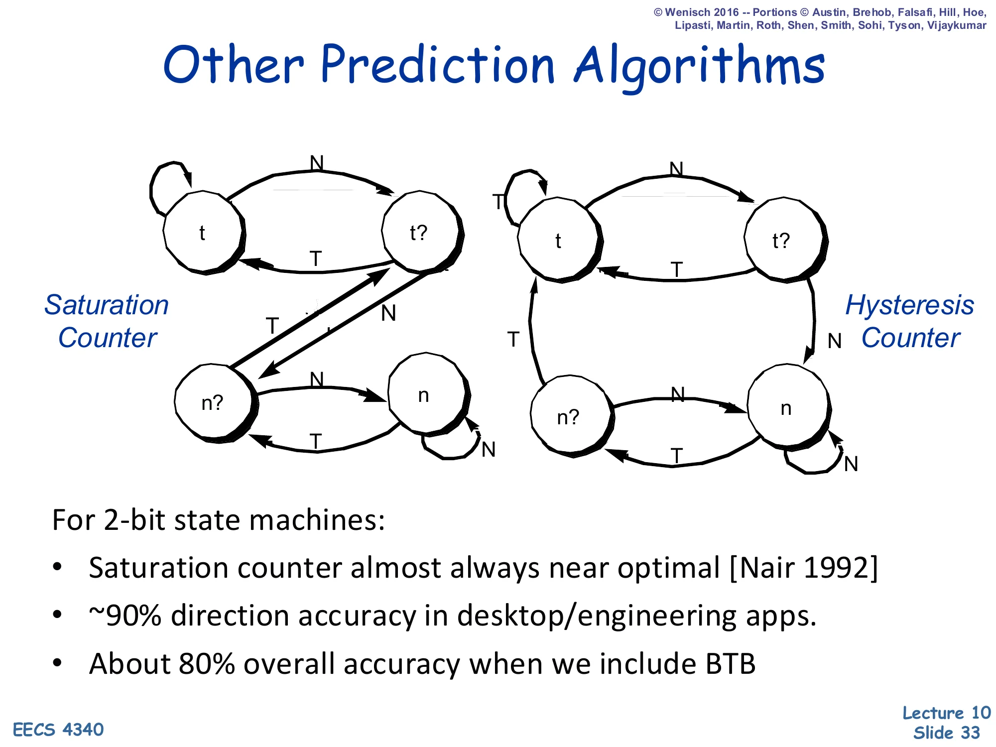
Two 2-bit FSMs side by side: a Saturation Counter and a Hysteresis Counter.

For 2-bit state machines:

• Saturation counter almost always near optimal [Nair 1992]
• ~90% direction accuracy in desktop/engineering apps
• About 80% overall accuracy when we include BTB

Among all four-state 2-bit FSMs, the saturation counter of slide 32 is empirically near-optimal — Nair (1992) compared every variant and showed the saturation policy minimizes mispredictions across SPEC-style workloads. An alternative, the hysteresis counter, treats the two middle states differently and ends up similar but slightly worse. The headline number is 90% direction accuracy on typical desktop and engineering applications, which sounds high but is far below modern requirements: with 20% branch frequency and a deep pipeline, even 90% direction accuracy means a misprediction every 50 instructions, and the BTB adds further losses, dragging combined accuracy to ~80%. Real systems need >95% direction accuracy, which is what the correlated, GShare, hybrid, and TAGE predictors on later slides aim to deliver.

Using More History: Correlated Predictor

Slide 34

Show slide text

Using More History: Correlated Predictor

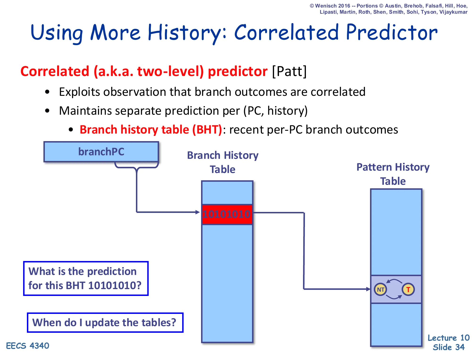
Correlated (a.k.a. two-level) predictor [Patt]

• Exploits observation that branch outcomes are correlated
• Maintains separate prediction per (PC, history)
  • Branch history table (BHT): recent per-PC branch outcomes

Diagram: branchPC selects a row of the BHT containing a recent outcome history (e.g., 10101010). That history indexes the Pattern History Table (PHT) of 2-bit counters, whose selected entry produces the prediction.

• What is the prediction for this BHT 10101010?
• When do I update the tables?

Yeh & Patt’s two-level / correlated predictor extends the BHT idea by keeping a recent outcome history per branch PC and using that history to index a second table — the Pattern History Table (PHT) — of 2-bit counters. The intuition is that many branches have outcomes correlated with their own recent past: a branch that produced N,T,T very often produces T next, even if the branch as a whole is not biased toward either direction. Each row of the BHT stores a $k$-bit shift register of recent outcomes (here 10101010), and the PHT has $2^k$ entries indexed by that register, each entry a 2-bit saturating counter. The slide ends with the two implementation questions answered later: when to update history (speculative update at fetch with rollback on misprediction) and how to manage the substantial PHT storage.

Correlated Predictor Example — Step 1

Slide 35

Show slide text

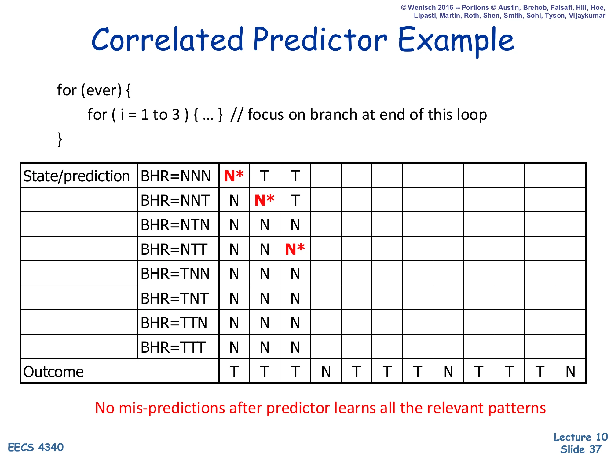
Correlated Predictor Example

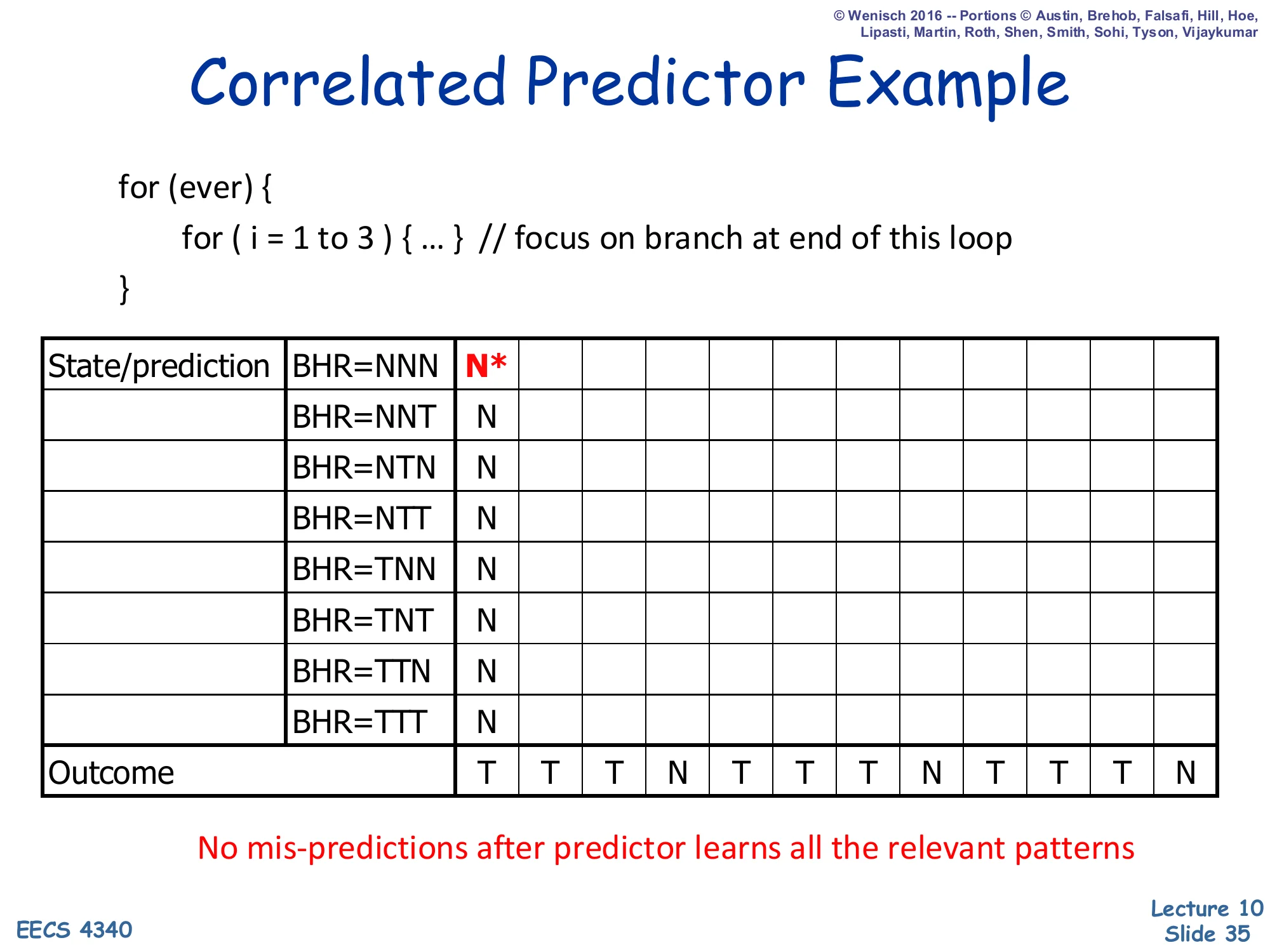
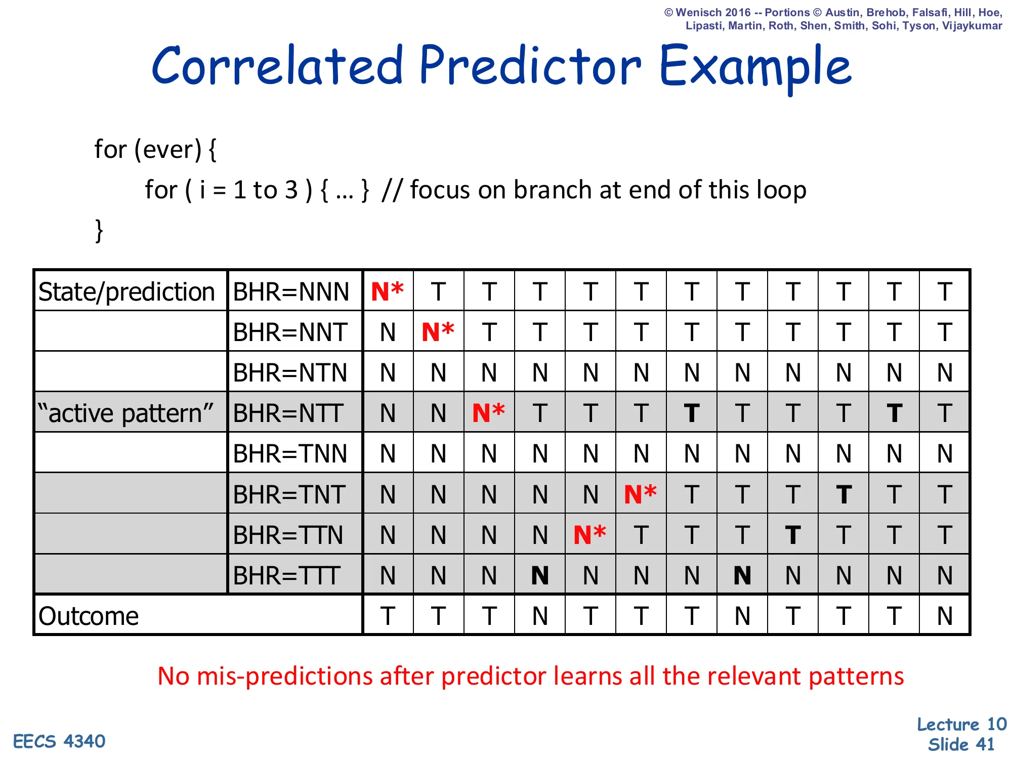
for (ever) {
    for (i = 1 to 3) { ... }   // focus on branch at end of this loop
}

State table: BHR rows ∈ {NNN, NNT, NTN, NTT, TNN, TNT, TTN, TTT}; each cell is the prediction at that step.

Step 1: BHR=NNN, prediction = N* (mis-predict). All other rows still N (initialized).

Outcome stream: T T T N T T T N T T T N — no mis-predictions after predictor learns all the relevant patterns.

Slides 35–41 walk through a 3-bit-history correlated predictor on the same for(i=1..3) inner loop from slide 31. The BHR (branch history register) has 8 possible patterns (NNN through TTT), each with its own 2-bit counter in the PHT — for clarity the slides show only the prediction bit. At step 1 the BHR is NNN and the prediction is N (mispredicting because the actual outcome is T). The promise highlighted in red — no mispredictions after predictor learns all the relevant patterns — is the central claim of correlated prediction: once each active BHR pattern has been visited and trained, the predictor predicts the correct outcome for that pattern every subsequent time, because the loop’s behavior is purely a function of the previous three outcomes.

Correlated Predictor Example — Step 2

Slide 36

Show slide text

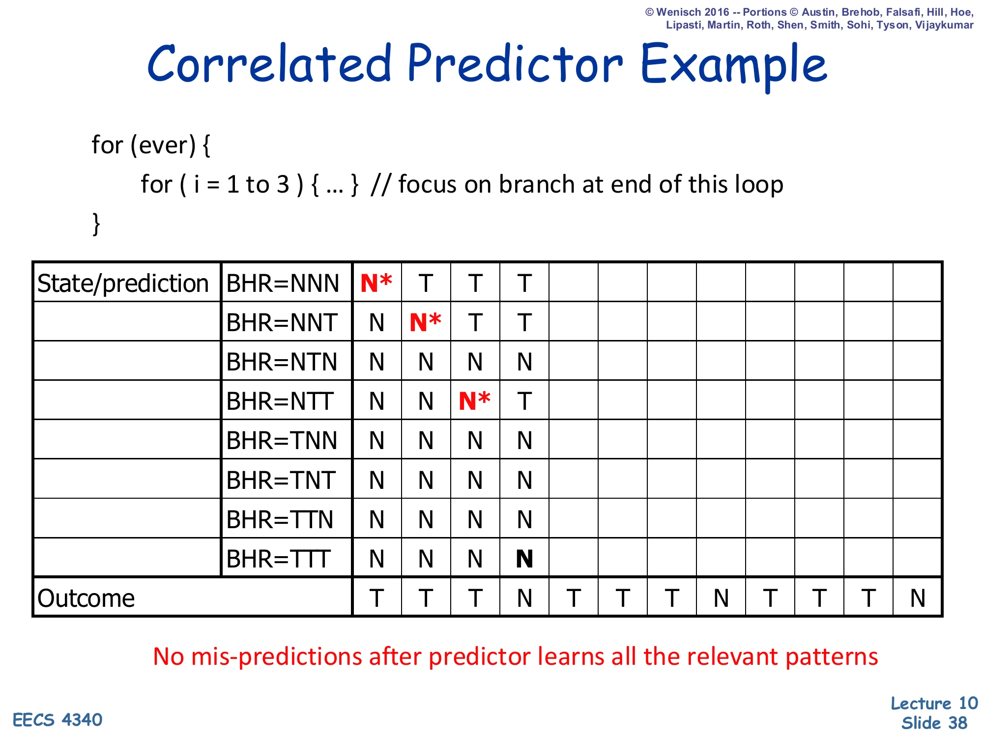
Correlated Predictor Example

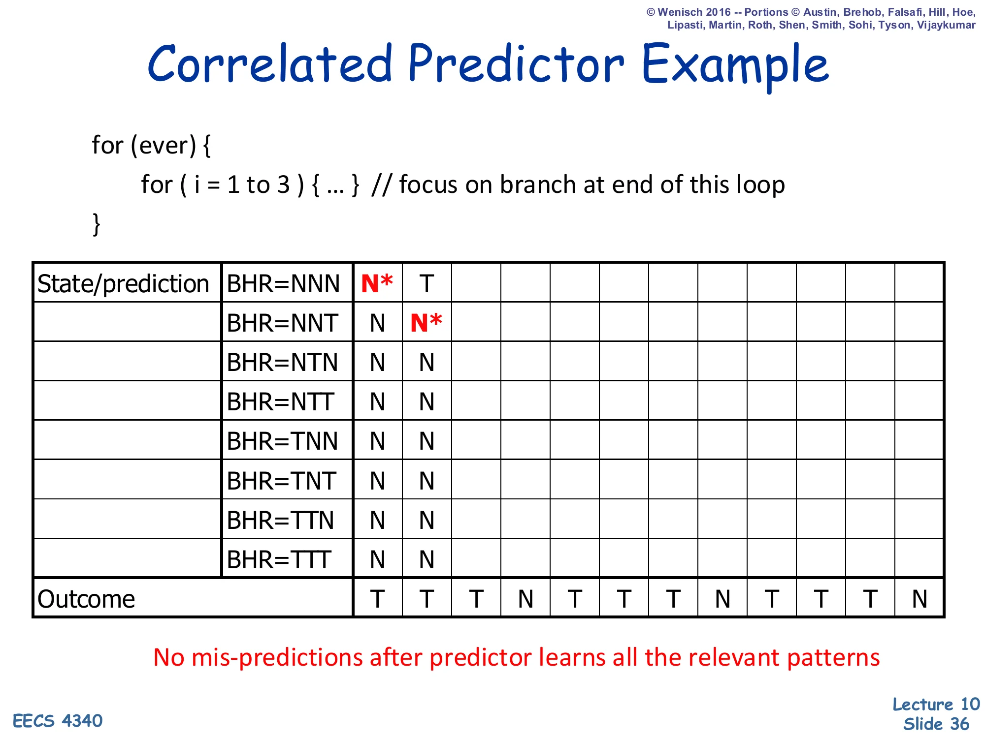
Step 2: After observing T at step 1, BHR shifts to NNT. Prediction at NNT = N* (mis-predict). NNN row updated to T.

Outcome stream so far: T T…

After step 1 the predictor learned that BHR=NNN→T (the cell is now T), and the BHR shifts to NNT for the next prediction. Step 2 again predicts N (default initialization) but the actual outcome is T, so this is the second misprediction. The active row updates to T. With each subsequent visit, the BHR rotates through the pattern’s reachable states and each row is corrected exactly once. Crucially, only a subset of the 8 possible BHR values are ever reached on this loop — the unreachable rows (e.g., NTN, TNN, TNT, TTN) keep their default N forever and don’t matter for accuracy. This is the active pattern idea highlighted on slide 41.

Correlated Predictor Example — Step 3

Slide 37

Show slide text

Correlated Predictor Example

Step 3: BHR now NTT after observing T,T. Prediction at NTT = N* (mis-predict). NNN updates to T (already), NNT updates to T.

Outcome stream so far: T T T…

Step 3: the third outcome is T, so the BHR has rotated to NTT. The predictor still has its default N at NTT and mispredicts the third T. After the update, both NNN→T and NNT→T are learned, and NTT is being trained. So far the predictor has missed three times (one per new BHR pattern visited), which is exactly the cost of warming up the relevant rows of the PHT. Unlike the simple BHT of slide 31, however, these misses do not recur on subsequent iterations — once a pattern is learned, it is learned for good (until interfering training corrupts it, which doesn’t happen in this regular loop).

Correlated Predictor Example — Step 4

Slide 38

Show slide text

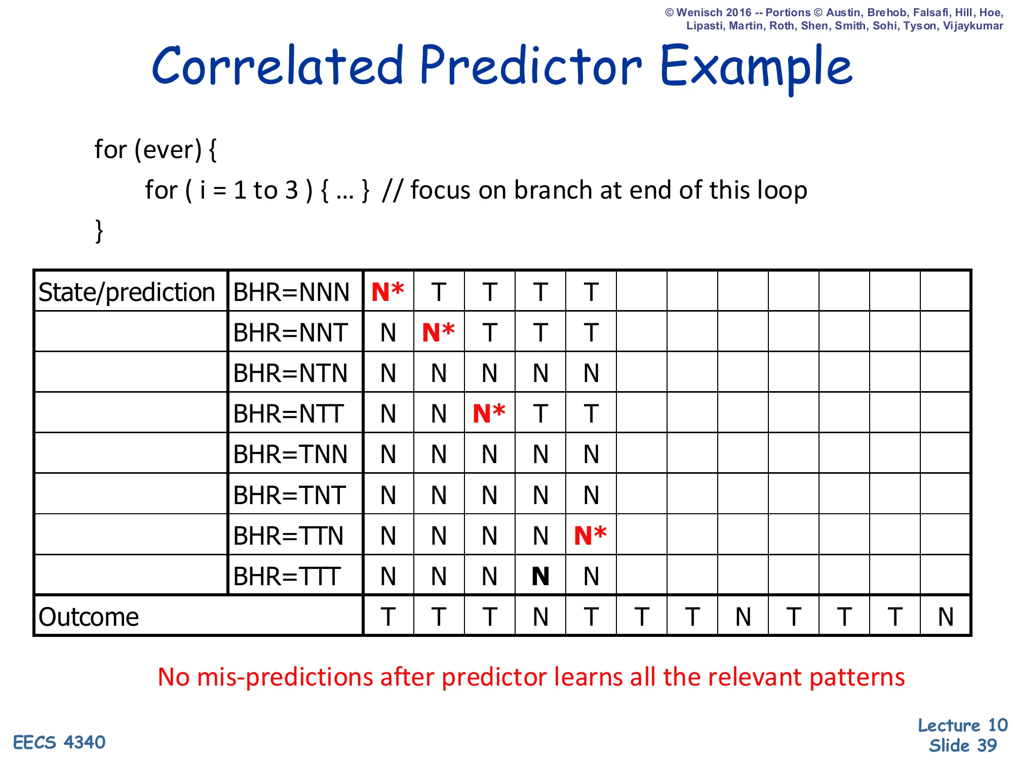
Correlated Predictor Example

Step 4: outcome at step 3 was T, BHR shifts to TTT. Prediction at TTT = N (correct! outcome = N — that’s the loop falling out). TTT row stays N (already correct). All trained rows now: NNN→T, NNT→T, NTT→T.

Step 4 is the first correct prediction. After three taken outcomes, the BHR is TTT, and the loop is now exiting (j reached 3), so the actual outcome is N. The default-initialized TTT row predicts N — coincidentally correct on the first visit. The active rows so far are NNN, NNT, NTT, TTT, with NNN→T, NNT→T, NTT→T, TTT→N. After this point, each subsequent iteration cycles through exactly these four BHR patterns and each prediction matches the trained outcome — which is why the slide insists no mispredictions after the predictor learns all the relevant patterns. The total warmup cost is just three mispredictions, after which every later prediction is correct.

Correlated Predictor Example — Step 5

Slide 39

Show slide text

Correlated Predictor Example

Step 5: BHR now TTN (after T,T,N). Prediction at TTN = N* (mis-predict — outcome is T). New mis-prediction column highlighted.

Step 5 introduces a fourth warmup miss: after the loop falls out and the outer loop starts the next iteration, the BHR is TTN (the last three outcomes: T, T, N), but the next outcome is T (the inner loop runs again). TTN was a default N, so the predictor mispredicts. After this update, TTN→T is trained. The picture so far: the only BHR rows that ever appear in the steady-state pattern of this nested loop are NNN, NNT, NTT, TTT, TTN — five out of eight possible rows. The remaining three (NTN, TNN, TNT) are never visited because the loop’s outcome stream TTTNTTTNTTTN… never produces them.

Correlated Predictor Example — Step 6

Slide 40

Show slide text

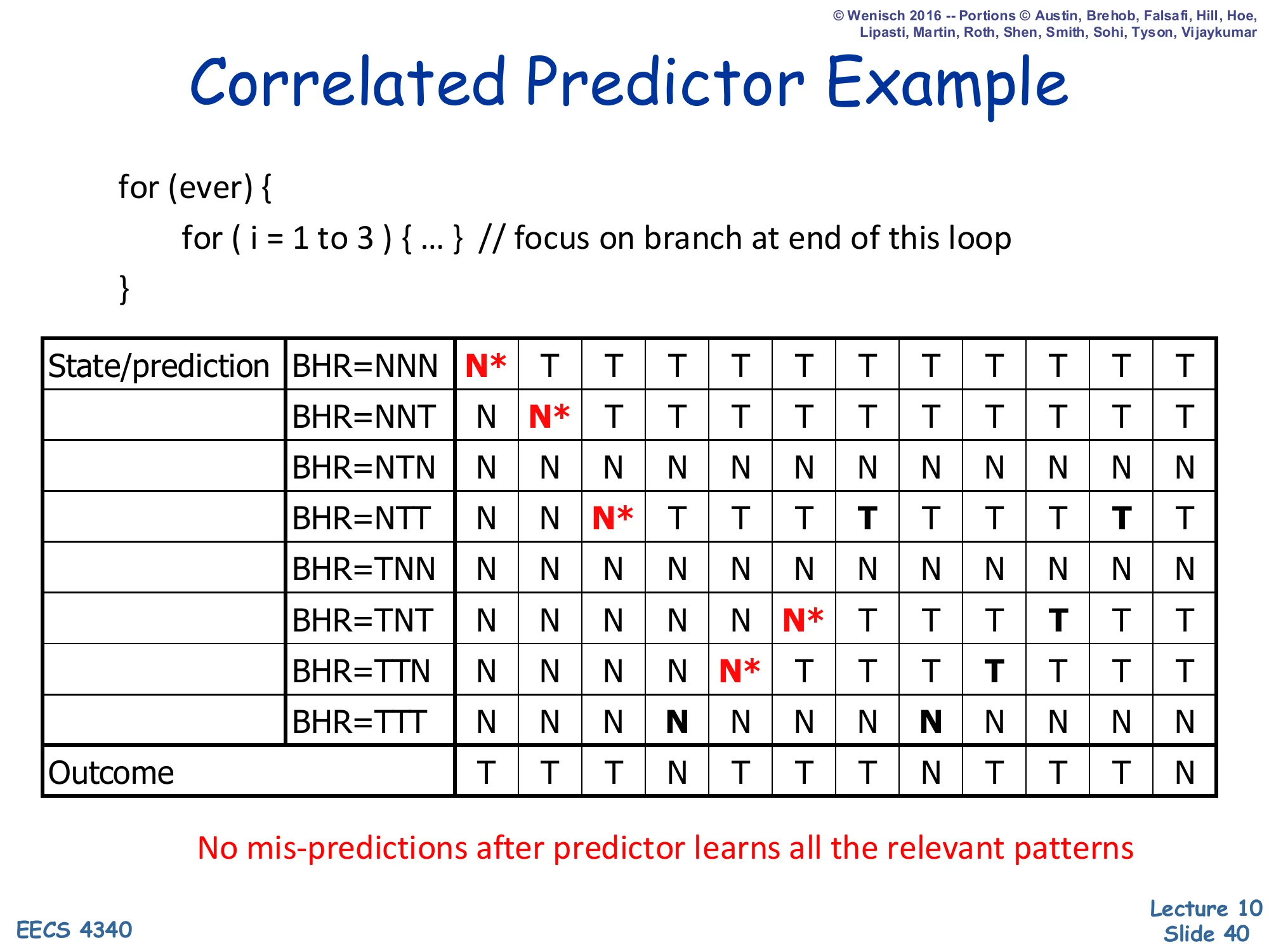
Correlated Predictor Example

Step 6: BHR has rotated through patterns. Final state shows TNT mis-predict (N* when outcome is T) is the next new pattern to train. After this iteration, all active rows are: NNN→T, NNT→T, NTT→T, TTT→N, TTN→T, TNT→T.

By step 6 the BHR has cycled through TTN→TNT and the predictor warms up TNT→T at the cost of one more misprediction. Counting all the warmup misses on the slide so far gives roughly one miss per new active BHR pattern — consistent with information theory: the predictor needs at least one observation per state to learn the conditional outcome distribution. After this final miss every subsequent prediction is correct. Compared with the simple BHT of slide 31 (two mispredictions per iteration of the outer loop, forever), the correlated predictor amortizes its warmup cost to zero over the lifetime of the loop. This is the core reason real CPUs use multi-bit history.

Correlated Predictor Example — Active Pattern

Slide 41

Show slide text

Correlated Predictor Example

The “active pattern” shaded rows are the BHR values actually visited by this loop: NTT, TNT, TTN, TTT (and, transiently during warmup, NNN and NNT).

No mis-predictions after predictor learns all the relevant patterns.

The final summary slide highlights the active pattern concept — only a small subset of the $2^k$ possible BHR values are ever indexed for any given branch. For the 3-iteration inner loop, the steady-state active set is just 4 rows out of 8 (NTT, TNT, TTN, TTT). This is design choice III on slide 44: most PHT rows are wasted because most BHR patterns never appear, which motivates separate per-PC PHTs (PAp/GAp configurations) so different branches can use the same shared BHR space with their own table. The deeper observation — that branches with $k$ bits of history can be perfectly predicted once the active patterns warm up — is the foundation for everything from GShare through TAGE.

Global Branch Prediction

Slide 42

Show slide text

Global Branch Prediction

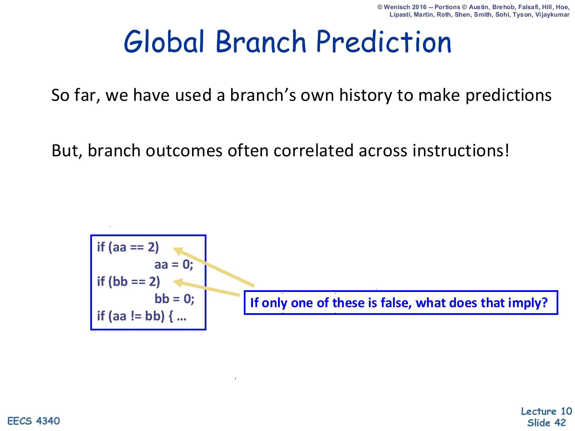
So far, we have used a branch’s own history to make predictions

But, branch outcomes often correlated across instructions!

if (aa == 2)
    aa = 0;
if (bb == 2)
    bb = 0;
if (aa != bb) { ...

If only one of these is false, what does that imply?

This slide makes the case for global (rather than per-PC) branch history. The example shows three branches whose outcomes are not independent: if aa==2 is true and the body sets aa=0, and bb==2 is false (so bb keeps its value), then the third branch aa != bb is guaranteed to take a particular direction — the outcomes are functionally correlated across different branch PCs. A per-PC predictor cannot exploit this because it only sees the third branch’s own history; a global predictor that records the outcomes of all recent branches in a single shared shift register can. The next slide describes the implementation: a global BHR shifted on every branch and used to index the PHT, capturing exactly this kind of inter-branch correlation.

Global Prediction Implementation

Slide 43

Show slide text

Global Prediction Implementation

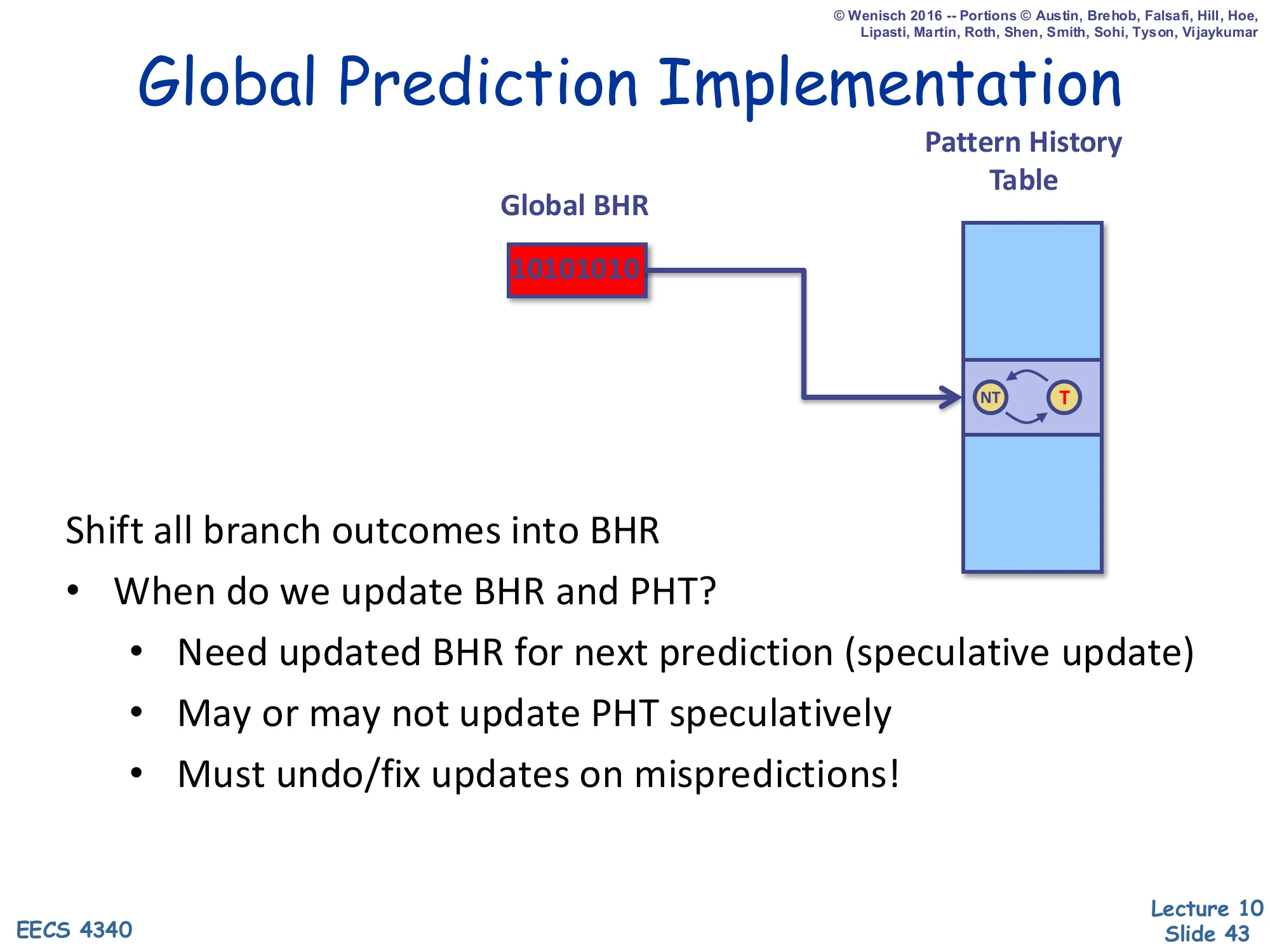
Diagram: a single Global BHR (e.g., 10101010) indexes a global Pattern History Table of 2-bit counters; the selected entry’s NT/T state is the prediction.

Shift all branch outcomes into BHR

• When do we update BHR and PHT?
  • Need updated BHR for next prediction (speculative update)
  • May or may not update PHT speculatively
  • Must undo/fix updates on mispredictions!

A global predictor uses one shift register — the Global BHR — that records the outcome of every branch, regardless of PC. The PHT is then indexed by that global history alone (or by combining it with the PC, as in GShare on slide 48). Two implementation subtleties: (1) the BHR must be speculatively updated at fetch time so the very next branch’s prediction sees the latest history — but the speculation must be undone on a misprediction by saving a snapshot of the BHR at every branch and restoring it during recovery; (2) the PHT may or may not be updated speculatively, with non-speculative updates avoiding the rollback cost at the price of occasionally training the predictor on stale history. These two issues are why real BPUs include checkpointing logic alongside the BHR/PHT.

Correlated Predictor Design Space

Slide 44

Show slide text

Correlated Predictor Design Space

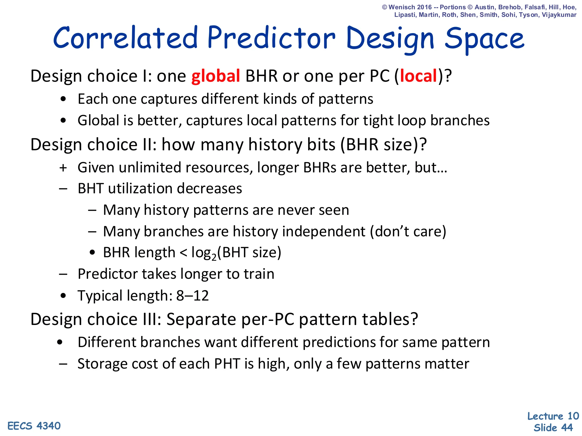
Design choice I: one global BHR or one per PC (local)?

• Each one captures different kinds of patterns
• Global is better, captures local patterns for tight loop branches

Design choice II: how many history bits (BHR size)?

• Given unlimited resources, longer BHRs are better, but…
• BHT utilization decreases
  • Many history patterns are never seen
  • Many branches are history independent (don’t care)
  • BHR length < $\log_2(\text{BHT size})$
• Predictor takes longer to train
• Typical length: 8–12

Design choice III: Separate per-PC pattern tables?

• Different branches want different predictions for same pattern
• Storage cost of each PHT is high, only a few patterns matter

The three correlated-predictor design choices map directly to the {G,P}A{g,p,s} taxonomy on the next slide. Choice I — global vs per-PC BHR — trades inter-branch correlation (global wins for code with cross-branch dependencies) against local correlation (per-PC wins for self-contained loops). The slide notes empirically that global is better even for tight loops because the global BHR still captures the local pattern as part of its longer history. Choice II — history length — rewards longer histories until two effects cap it: most BHR patterns are never visited (the active pattern observation from slide 41), and longer histories take more iterations to train. Typical 8–12 bits balances these. Choice III — global vs per-PC vs per-set PHT — addresses destructive aliasing: two branches that prefer opposite outcomes for the same BHR pattern destroy each other’s training in a shared PHT, but separate per-PC PHTs are too expensive.

Taxonomy & Nomenclature [Patt]

Slide 45

Show slide text

Taxonomy & Nomenclature [Patt]

Diagram: branchPC indexes per-PC BHRs (each row a recent history); the selected BHR indexes a per-PC PHT to produce the 2-bit-counter prediction.

${G,P}A{g,p,s}$ naming convention:

• First letter (uppercase): Global or Per-PC BHR
• Middle letter A = “Adaptive”
• Third letter (lowercase): global, per-PC, or set PHT

Yeh & Patt’s taxonomy describes any two-level predictor with a 4-character name {G,P}A{g,p,s}. The leading letter says how branch history is partitioned: Global means a single shared BHR for all branches; Per-PC means one BHR per branch PC. The middle A stands for Adaptive. The trailing letter says how the PHT is partitioned: global (one shared PHT), per-PC (one PHT per branch), or set (per-set PHTs, somewhere in between). So GAg is global-BHR + global-PHT (very small storage, prone to aliasing), PAp is per-PC-BHR + per-PC-PHT (huge storage, no aliasing), and the slides 46–47 work through PAg/PAs/PAp and GAg/GAs/GAp side by side. GShare on slide 48 is essentially a clever GAg variant that XORs PC into the BHR index to reduce destructive aliasing.

Per-PC History

Slide 46

Show slide text

Per-PC History

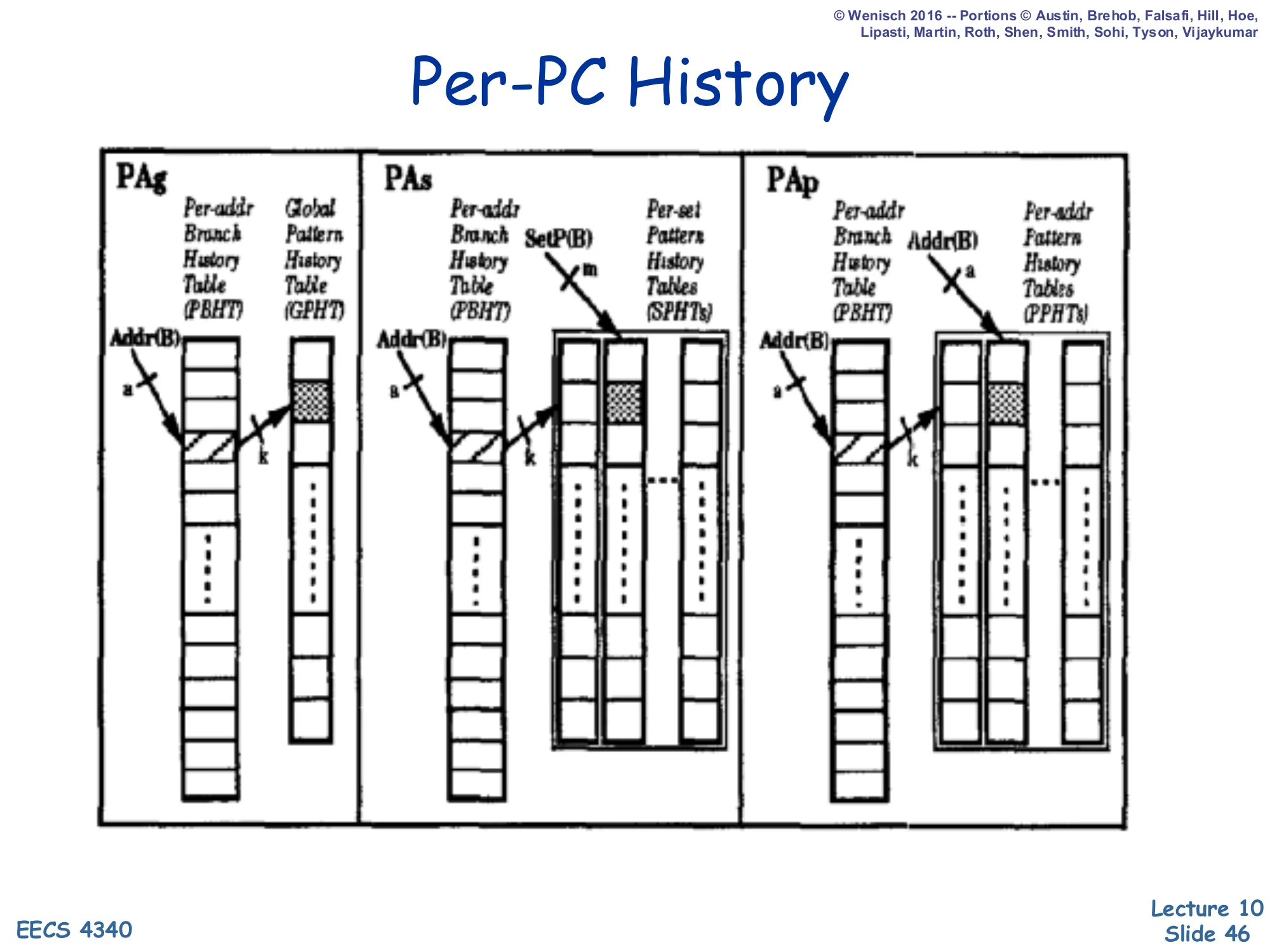
Three configurations (PAg, PAs, PAp) shown side by side:

• PAg: Per-Address Branch History Table (PBHT) → Global Pattern History Table (GPHT)
• PAs: Per-Address BHT → per-Set Pattern History Tables (SPHTs); SetP(B) selects which set
• PAp: Per-Address BHT → Per-Address PHTs (PPHTs); Addr(B) selects which PHT

These three configurations all use a per-PC BHR (the leading P) but differ in PHT organization. PAg shares one global PHT across all branches — cheap storage but maximum destructive aliasing because two PCs whose BHRs happen to hold the same pattern will collide on the same counter. PAs allocates one PHT per set of PCs, reducing aliasing at the cost of more storage. PAp goes all the way to one PHT per PC — no aliasing at all but storage explodes as the product of (number of branches) × $2^k$. In practice, PAg is the workhorse: with reasonable BHR length and PHT size, the destructive aliasing is small, and the area savings are huge. A purely per-PC BHR is good at capturing self-contained loops but misses inter-branch correlations like the aa/bb example on slide 42.

Global History

Slide 47

Show slide text

Global History

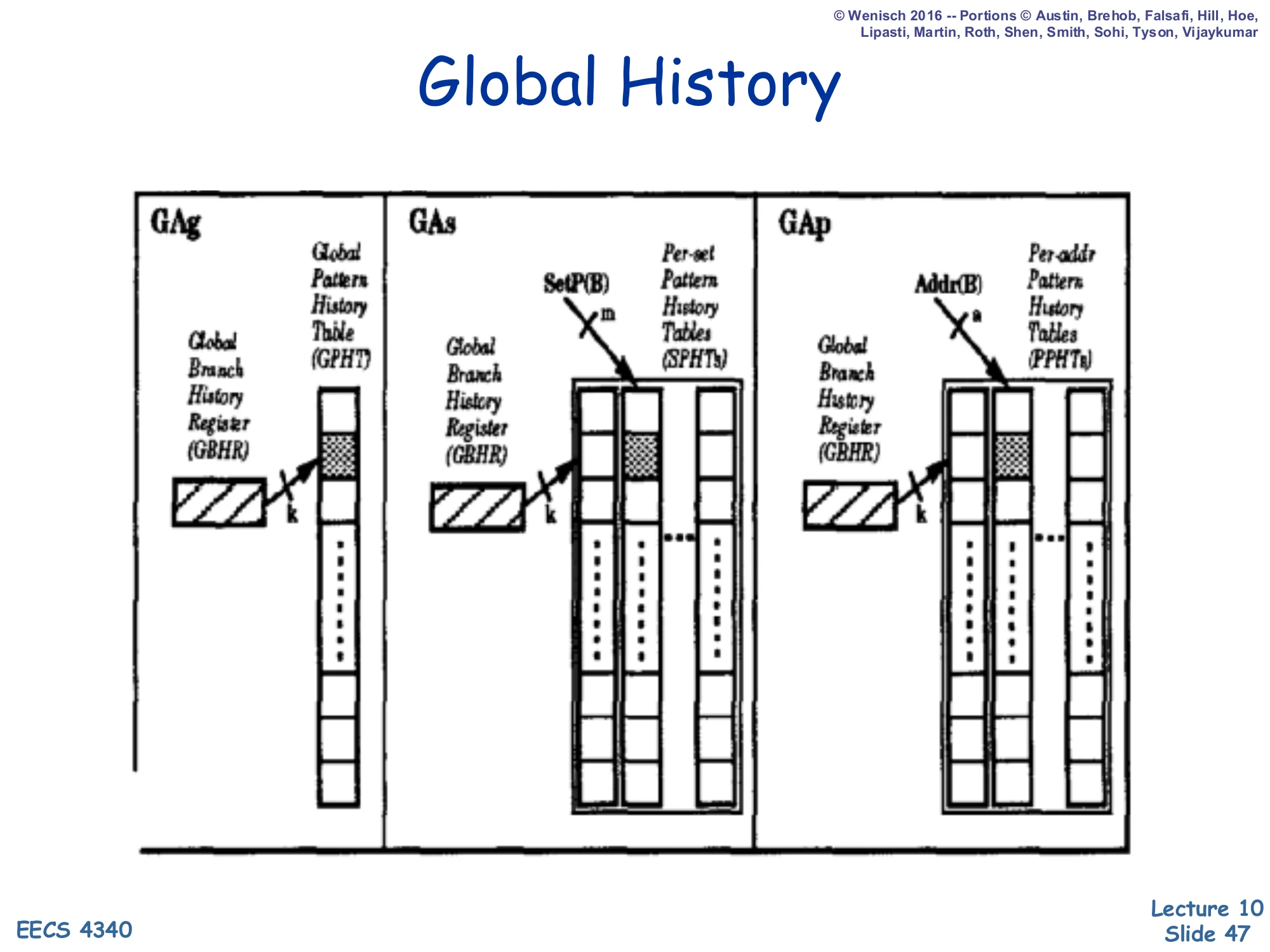
Three configurations (GAg, GAs, GAp) shown side by side:

• GAg: Global BHR (GBHR) → Global PHT (GPHT)
• GAs: GBHR → per-Set PHTs (SPHTs); SetP(B) selects the set
• GAp: GBHR → Per-Address PHTs (PPHTs); Addr(B) selects the PHT

These are the global-BHR analogs of the previous slide. GAg is the simplest two-level global predictor — one shared GBHR feeds one shared PHT — and it captures inter-branch correlations cheaply but again suffers from PHT aliasing. GAs and GAp progressively partition the PHT by set or by PC to reduce aliasing at the cost of more storage. GShare (next slide) is the practical sweet spot: it uses a global BHR (catching inter-branch correlation) but indexes a global PHT with BHR XOR PC, getting most of the benefit of per-PC PHTs without the storage cost. Most modern direction predictors evolved from this lineage — TAGE, perceptron, and hashed-index variants are all elaborations of the GAg/GAp design space.

Gshare [McFarling]

Slide 48

Show slide text

Gshare [McFarling]

Diagram: branchPC and Global BHR (e.g., 10101010) are XORed; the result indexes a global PHT of 2-bit counters whose selected entry yields the NT/T prediction.

Cheap way to implement GAs

• Global branch history
• Per-address patterns (sort of)
• Try to make the PHT big enough to avoid collisions

GShare (McFarling, 1993) is the most influential dynamic direction predictor in the lecture. It uses a single global BHR for inter-branch correlation, but instead of indexing the global PHT directly with the BHR (GAg, prone to aliasing), it XORs the BHR with the branch PC and uses the result as the PHT index. This single XOR achieves a cheap approximation of per-PC PHTs: two branches with the same recent global history but different PCs produce different indices, so they don’t share a counter — exactly the destructive-aliasing problem GAg suffered from. The slide’s three bullets summarize the design as global-history + per-address-patterns (sort of) + a sufficiently large PHT to keep collisions low. GShare is the direction-prediction half of the Alpha 21264 hybrid predictor on the next slide.

Hybrid (Tournament) Predictor

Slide 49

Show slide text

Hybrid Predictor

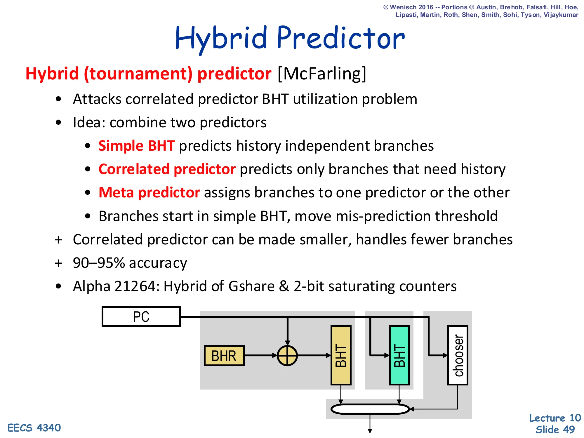
Hybrid (tournament) predictor [McFarling]

• Attacks correlated predictor BHT utilization problem
• Idea: combine two predictors
  • Simple BHT predicts history independent branches
  • Correlated predictor predicts only branches that need history
  • Meta predictor assigns branches to one predictor or the other
  • Branches start in simple BHT, move mis-prediction threshold

• Correlated predictor can be made smaller, handles fewer branches
• 90–95% accuracy

• Alpha 21264: Hybrid of Gshare & 2-bit saturating counters

Diagram: PC and BHR feed two predictors in parallel — one BHT (PC-only), one BHT indexed by PC XOR BHR — and a chooser (meta-predictor) selects between them.

A hybrid (tournament) predictor combines two predictors with complementary strengths and a meta-predictor that learns which one to trust per branch. The simple BHT (or 2-bit counter table) predicts history-independent branches well and uses storage efficiently because every entry contributes; the correlated/GShare predictor handles the harder branches that need history. The meta-predictor (the chooser) is typically itself a small 2-bit counter table indexed by PC: it tracks which of the two predictors has been more accurate for each branch and routes the prediction accordingly. A new branch starts in the simple BHT and only migrates to the correlated predictor once mispredictions exceed a threshold. The Alpha 21264 — the canonical hybrid example — combines GShare and 2-bit saturating counters and reaches 90–95% direction accuracy.

Towards the State of the Art: TAGE

Slide 50

Show slide text

Towards the state of the art: TAGE [Seznec]

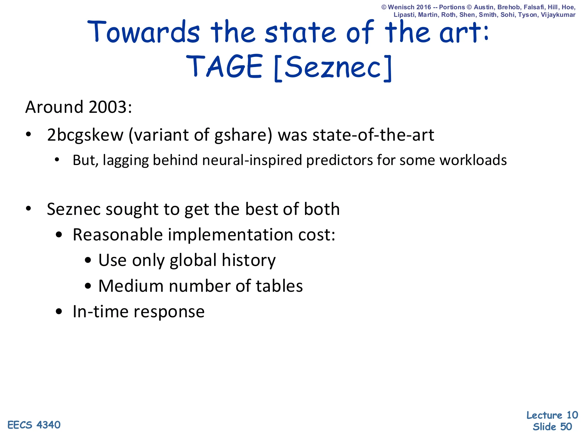
Around 2003:

• 2bcgskew (variant of gshare) was state-of-the-art

  • But, lagging behind neural-inspired predictors for some workloads

• Seznec sought to get the best of both

  • Reasonable implementation cost:
    • Use only global history
    • Medium number of tables
  • In-time response

By the early 2000s, GShare variants like 2bcgskew were the practical state of the art but were being beaten in academic competitions by perceptron-based (neural-inspired) predictors that were unimplementable in real silicon timing budgets. Seznec’s TAGE (TAgged GEometric history length) split the difference: it sticks to global history (cheaper than per-PC) and uses a moderate number of tables (cheaper than perceptrons), but achieves accuracy approaching neural predictors. The two main innovations: (1) multiple PHTs indexed by geometrically increasing history lengths so different tables specialize in branches with different history-length needs, and (2) tagged entries so that a table only provides a prediction when its history actually matches the current branch — overriding a default base predictor. TAGE remains the basis for most modern industrial direction predictors (e.g., AMD Zen, ARM Cortex).

TAGE: Multiple-Length Global History

Slide 51

Show slide text

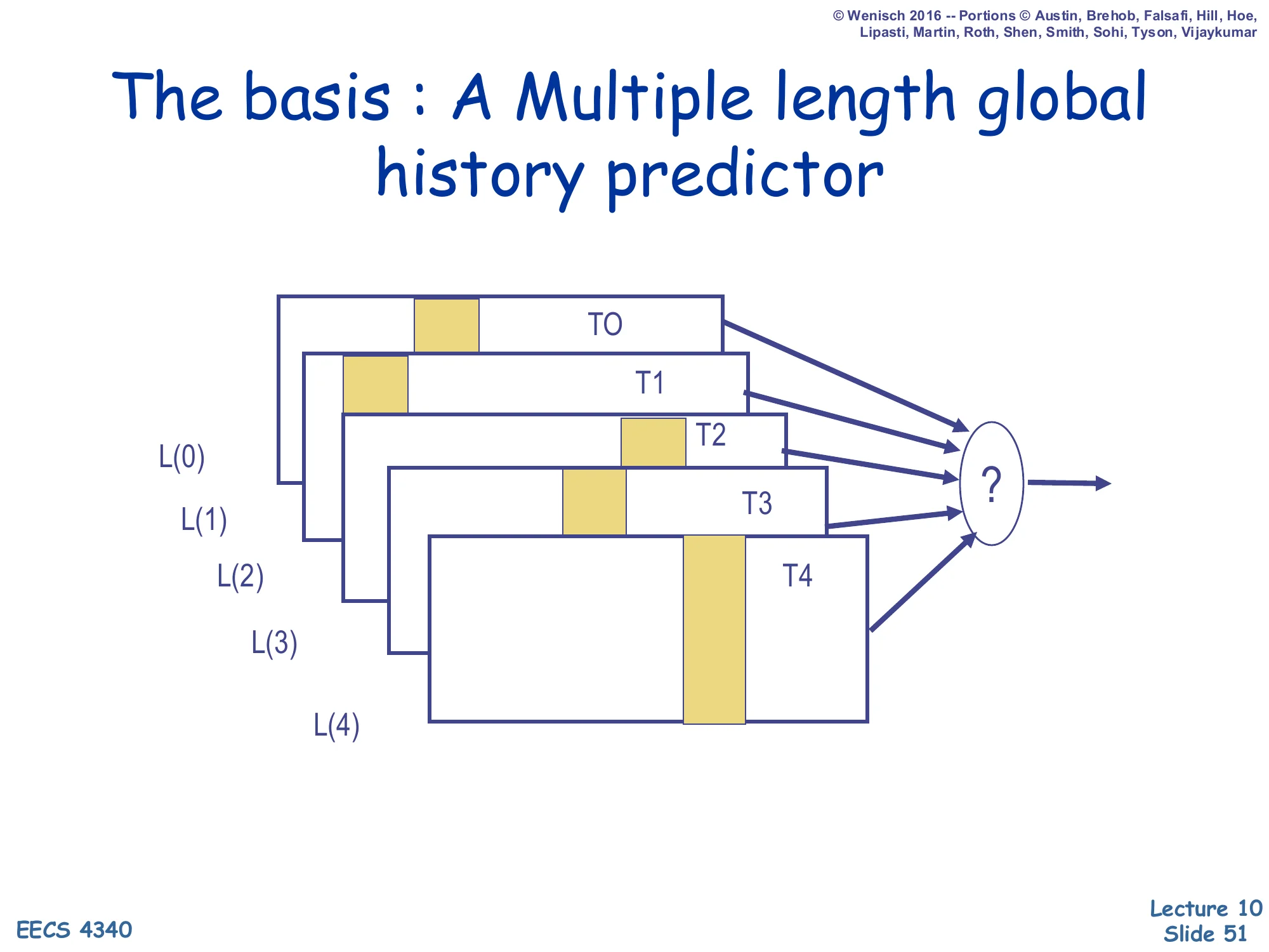
The basis: A Multiple length global history predictor

Diagram: tables T0…T4 fed by history lengths $L(0) < L(1) < L(2) < L(3) < L(4)$, each contributing a prediction, with a final selector ”?”.

TAGE’s core insight is that different branches need different amounts of history to be predictable. A simple loop branch needs only a few bits; a branch deep inside a complex correlated chain may need 50+ bits. Rather than picking one history length, TAGE keeps multiple PHTs T0…T4 indexed by geometrically increasing history lengths (e.g., $L(0)=0, L(1)=4, L(2)=12, L(3)=32, L(4)=80$). On a prediction the predictor consults all tables in parallel and the selector picks the prediction from the longest-history table that has a tag-matching entry. T0 is the base predictor that always provides a default (typically a 2-bit counter BHT), so a prediction is always available even when no longer-history table tags match.

TAGE Tagged Tables Implementation

Slide 52

Show slide text

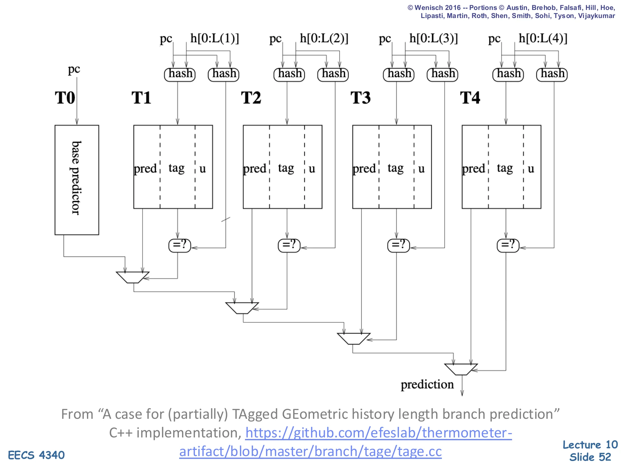
TAGE Implementation

Diagram: PC + history $h[0:L(i)]$ feed two hash functions per table $T_i, i \in \{1..4\}$ — one produces the index, the other produces the tag. Each entry has fields pred | tag | u. Tag-match comparators feed a chain of MUXes that select the longest matching table’s prediction; T0 (base predictor) is the fallback.

From “A case for (partially) TAgged GEometric history length branch prediction”. C++ implementation: https://github.com/efeslab/thermometer-artifact/blob/master/branch/tage/tage.cc

TAGE’s full implementation has four key features visible in this diagram. (1) Each tagged table $T_i$ has its own hash function that mixes PC with the first $L(i)$ bits of global history, producing both an index and a tag. (2) Each entry stores three fields: a prediction counter (pred), a partial tag (tag), and a usefulness counter (u) used by the replacement policy. (3) On prediction, every table is probed in parallel; the longest-history table with a tag match wins, and its pred counter produces the final taken/not-taken prediction. (4) On training, the winning table updates pred, and on misprediction TAGE may allocate a new entry in a longer-history table to learn the previously-missing pattern. The combination of geometric histories, partial tagging, and selective allocation is what gives TAGE its near-neural accuracy with FPGA-implementable timing — and the open-source C++ reference is the same code used by recent papers like Thermometer.

Readings (repeat)

Slide 53

Show slide text

Readings

For today:

• H & P Chapter 3.3
• A comparison of dynamic branch predictors that use two levels of branch history — https://dl.acm.org/doi/abs/10.1145/165123.165161

For next Monday:

• H & P Chapter 3.9
• McFarling: Combining Branch Predictors

Announcements (repeat)

Slide 54

Show slide text

Announcements

Project #4

• Due: milestone 3, 8-April-26
• In-person mandatory project check-in
  • 8:40–8:50 AM: CCDYMP
  • 8:50–9:00 AM: G13
  • 9:00–9:10 AM: GaPiChiXuXu
  • 9:10–9:20 AM: OoO
  • 9:20–9:30 AM: RISCy Whisky
  • 9:30–9:40 AM: SIX
  • 9:40–9:50 AM: UNI

Optional project meetings

• Mondays and Wednesdays during my office hours

https://courseworks2.columbia.edu/courses/237081